
10. Annex C: Reliability Analysis Principles#
10.1. Introduction#
In recent years, practical reliability methods have been developed to help engineers tackle the analysis, quantification, monitoring and assessment of structural risks, undertake sensitivity analysis of inherent uncertainties and make appropriate decisions about the performance of a structure. The structure may be at the design stage, under construction or in actual use.
This Annex C summarizes the principles and procedures used in formulating and solving risk related problems via reliability analysis. It is neither as broad nor as detailed as available textbooks on this subject, some of which are included in the bibliography. Its purpose is to underpin the updating and decision-making methodologies presented in part 2 of this document.
Starting from the principles of limit state analysis and its application to codified design, the link is made between unacceptable performance and probability of failure. It is important, especially in assessment, to distinguish between components and systems. System concepts are introduced and important results are summarized. The steps involved in carrying out a reliability analysis, whose main objective is to estimate the failure probability, are outlined and alternative techniques available for such an analysis are presented. Some recommendations on formulating stochastic models for commonly used variables are also included.
10.2. Concepts#
10.2.1. \(\underline{\text {Limit States}}\)#
The structural performance of a whole structure or part of it may be described with reference to a set of limit states which separate acceptable states of the structure from unacceptable states. The limit states are divided into the following two categories:
ultimate limit states, which relate to the maximum load carrying capacity.
serviceability limit states, which relate to normal use.
The boundary between acceptable (safe) and unacceptable (failure) states may be distinct or diffuse but, at present, deterministic codes of practice assume the former. Thus, verification of a structure with respect to a particular limit state is carried out via a model describing the limit state in terms of a function (called the limit state function) whose value depends on all relevant design parameters. In general terms, attainment of the limit state can be expressed as:
where \(\mathbf{s}\) and \(\mathbf{r}\) represent sets of load (actions) and resistance variables. Conventionally, \(g(\mathbf{s}, \mathbf{r}) \leq 0\) represents failure; in other words, an adverse state.
The limit state function, \(g(\mathbf{s}, \mathbf{r})\), can often be separated into one resistance function, \(r(.)\), and one loading (or action effect) function, \(s(.)\) , in which case equation (10.1) can be expressed as:
10.2.2. \(\underline{\text{Structural Reliability}}\)#
Load, material and geometry parameters are subject to uncertainties, which can be classified according to their nature, see section 3. They can, thus, be represented by random variables (this being the simplest possible probabilistic representation, whereas more advanced models might be appropriate in certain situations, such as random fields). The variables \(\mathbf{S}\) and \(\mathbf{R}\) are often referred to as “basic random variables” (where the upper case letter is used for denoting random variables) and may be collectively represented by a random vector \(\mathbf{X}\).
In this context, failure is a probabilistic event and its probability of occurrence, \(P_{f}\), is given by:
where, \(M=g(\mathbf{X})\). Note that \(M\) is also a random variable, called the safety margin.
If the limit state function is expressed in the form of (10.2), (10.3) can be written as
where \(R=r~(\mathbf{R})\) and \(S=s~(\mathbf{S})\) are random variables associated with resistance and loading respectively. This expression is useful in the context of the discussion in section 2.2 on code formats and partial safety factors but will not be further used herein.
The failure probability defined in eqn (10.3) can also be expressed as follows:
where \(f_{\mathbf{X}}(\mathbf{x})\) is the joint probability density function of \(\mathbf{X}\).
The reliability, \(P_{S}\), associated with the particular limit state considered is the complementary event, i.e.
In recent years, a standard reliability measure, the reliability index \(\beta\), has been adopted which has the following relationship with the failure probability
where \(\Phi^{-1}(.)\) is the inverse of the standard normal distribution function, see Table 10.1
\(P_{f}\) |
\(10^{-1}\) |
\(10^{-2}\) |
\(10^{-3}\) |
\(10^{-4}\) |
\(10^{-5}\) |
\(10^{-6}\) |
\(10^{-7}\) |
|---|---|---|---|---|---|---|---|
\(\beta\) |
1.3 |
2.3 |
3.1 |
3.7 |
4.2 |
4.7 |
5.2 |
In most engineering applications, complete statistical information about the basic random variables \(\mathbf{X}\) is not available and, furthermore, the function \(g(.)\) is a mathematical model which idealizes the limit state. In this respect, the probability of failure evaluated from eqn (10.3) or (10.4) is a point estimate given a particular set of assumptions regarding probabilistic modelling and a particular mathematical model for \(g(.)\). The uncertainties associated with these models can be represented in terms of a vector of random parameters \(\mathbf{Q}\), and hence the limit state function may be re-written as \(g(\mathbf{X}, \mathbf{Q})\). It is important to note that the nature of uncertainties represented by the basic random variables \(\mathbf{X}\) and the parameters \(\mathbf{Q}\) is different. Whereas uncetainties in \(\mathbf{X}\) cannot be influenced without changing the physical characteristics of the problem (e.g. changing the steel grade), uncertainties in \(\mathbf{Q}\) can be influenced by the use of alternative methods and collection of additional data.
In this context, eqn (10.4) may be recast as follows
where \(P_{f}(\boldsymbol{\theta})\) is the conditional probability of failure for a given set of values of the parameters \(\boldsymbol{\theta}\) and \(f_{\mathbf{X} \mid \Theta}~(\mathbf{x} \mid \boldsymbol{\theta})\) is the conditional probability density function of \(\mathbf{X}\) for given \(\boldsymbol{\theta}\).
In order to account for the influence of parameter uncertainty on failure probability, one may evaluate the expected value of the conditional probability of failure, i.e.
where \(f_{\theta}(\theta)\) is the joint probability density function of \(\theta\). The corresponding reliability index is given by
The main objective of reliability analysis is to estimate the failure probability (or, the reliability index). Hence, it replaces the deterministic safety check with a probabilistic assessment of the safety of the structure, e.g. eqn (10.3) or eqn (10.8). Depending on the nature of the limit state considered, the uncertainty sources and their implications for probabilistic modeling, the characteristics of the calculation model and the degree of accuracy required, an appropriate methodology has to be developed. In many respects, this is similar to the considerations made in formulating a methodology for deterministic structural analysis but the problem is now set in a probabilistic framework.
10.2.3. \(\underline{\text{System Concepts}}\)#
Structural design is, at present, primarily concerned with component behaviour. Each limit state equation is, in most cases, related to a single mode of failure of a single component.
However, most structures are an assembly of structural components and even individual components may be susceptible to a number of possible failure modes. In deterministic terms, the former can be tackled through a progressive collapse analysis (particularly appropriate in redundant structures), whereas the latter is usually dealt with by checking a number of limit state equations.
However, the system behaviour of structures is not well quantified in limit state codes and requires considerable innovation and initiative from the engineer. A probabilistic approach provides a better platform from which system behaviour can be explored and utilised. This can be of benefit in assessment of existing structures where strength reserves due to system effects can alleviate the need for expensive strengthening.
There are two fundamental systems, see Fig. 10.1:
A series system is a system which fails if one or more of its components fail.
A parallel system is a system which fails when all its components have failed.
The probability of system failure is given by
where \(\mathrm{E}_{i}(i=1, \ldots n)\) is the event corresponding to failure of the \(i\) th component. In the case of parallel systems, which are designed to provide some redundancy, it is important to define the state of the component after failure. In structures, this can be described in terms of a characteristic load-displacement response, see Fig. 10.2, for which two convenient idealisations are the ‘brittle’ and the ‘fully ductile’ case. Intermediate, often more realistic, cases can also be defined.
The above expressions can be difficult to evaluate in the case of large systems with stochastically dependent components and, for this reason, upper and lower bounds have been developed, which may be used in practical applications. In order to appreciate the effect of system behaviour on failure probabilities, results for two special systems comprising equally correlated components with the same failure probability for each component are shown in Fig. 10.3(a) and Fig. 10.3(b). Note that in the case of the parallel system, it is assumed that the components are fully ductile.
More general systems can be constructed by combining the two fundamental types. It is fair to say that system methods are more developed for skeletal rather than continuous structures. Important results from system reliability theory are summarized in section 4.
10.3. Component Reliability Analysis#
The framework for probabilistic modeling and reliability evaluation is outlined in this section. The focus is on the procedure to be followed in assessing the reliability of a critical component with respect to a particular failure mode.
10.3.1. \(\underline{\text{General Steps}}\)#
The main steps in a component reliability analysis are the following:
select appropriate limit state function
specify appropriate time reference
identify basic variables and develop appropriate probabilistic models
compute reliability index and failure probability
perform sensitivity studies
Step (1) is essentially the same as for deterministic analysis. Step (2) should be considered carefully, since it affects the probabilistic modeling of many variables, particularly live loading. Step (3) is perhaps the most important because the considerations made in developing the probabilistic models have a major effect on the results obtained, see section 3.2. Step (4) should be undertaken with one of the methods summarized in section 3.3, depending on the application. Step (5) is necessary insofar as the sensitivity of any results (deterministic or probabilistic) should be assessed before a decision is taken.
10.3.2. \(\underline{\text{Probabilistic Modelling}}\)#
For the particular failure mode under consideration, uncertainty modeling must be undertaken with respect to those variables in the corresponding limit state function whose variability is judged to be important (basic random variables). Most engineering structures are affected by the following types of uncertainty:
intrinsic physical or mechanical uncertainty; when considered at a fundamental level, this uncertainty source is often best described by stochastic processes in time and space, although it is often modelled more simply in engineering applications through random variables.
measurement uncertainty; this may arise from random and systematic errors in the measurement of these physical quantities
statistical uncertainty; due to reliance on limited information and finite samples
model uncertainty; related to the predictive accuracy of calculation models used
The physical uncertainty in a basic random variable is represented by adopting a suitable probability distribution, described in terms of its type and relevant distribution parameters. The results of the reliability analysis can be very sensitive to the tail of the probability distribution, which depends primarily on the type of distribution adopted. A proper choice of distribution type is therefore important.
For most commonly encountered basic random variables there have been studies (of varying detail) that contain guidance on the choice of distribution and its parameters. If direct measurements of a particular quantity are available, then existing, so-called a priori, information (e.g. probabilistic models found in published studies) should be used as prior statistics with a relatively large equivalent sample size \(`\left(n^{\prime} \approx 50\right)\).
The following comments may also be helpful in selecting a suitable probabilistic model.
\(\underline{\text{Material properties}}\)
frequency of negative values is normally zero
log-normal distribution can often be used
distribution type and parameters should, in general, be derived from large homogeneous samples and with due account of established distributions for similar variables (e.g. for a new high strength steel grade, the information on properties of existing grades should be consulted); tests should be planned so that they are, as far as possible, a realistic description of the potential use of the material in real applications.
\(\underline{\text{Geometric parameters}}\)
variability in structural dimensions and overall geometry tends to be small
dimensional variables can be adequately modelled by the normal or log-normal distribution
if the variable is physically bounded, a truncated distribution may be appropriate (e.g. location of reinforcement); such bounds should always be carefully considered to avoid entering into physically inadmissible ranges
variables linked to manufacturing can have large coefficients of variation (e.g. imperfections, misalignments, residual stresses, weld defects).
\(\underline{\text{Load variables}}\)
loads should be divided according to their time variation (permanent, variable, accidental)
in certain cases, permanent loads consist of the sum of many individual elements; they may be represented by a normal distribution
for single variable loads, the form of the point-in-time distribution is seldom of immediate relevance; often the important random variable is the magnitude of the largest extreme load that occurs during a specified reference period for which the probability of failure is calculated (e.g. annual, lifetime)
the probability distribution of the largest extreme could be approximated by one of the asymptotic extreme-value distributions (Gumbel, sometimes Frechet)
when more than one variable loads act in combination, load modelling is often undertaken using simplified rules suitable for FORM/SORM analysis.
In selecting a distribution type to account for physical uncertainty of a basic random variable afresh, the following procedure may be followed:
based on experience from similar type of variables and physical knowledge, choose a set of possible distributions
obtain a reasonable sample of observations ensuring that, as far as possible, the sample points are from a homogeneous group (i.e. avoid systematic variations within the sample) and that the sampling reflects potential uses and applications
evaluate by an appropriate method the parameters of the candidate distributions using the sample data; the method of maximum likelihood is recommended but evaluation by alternative methods (moment estimates, least-square fit, graphical methods) may also be carried out for comparison.
compare the sample data with the resulting distributions; this can be done graphically (histogram vs. pdf, probability paper plots) or through the use of goodness-of-fit tests (Chi-square, Kolmogorov-Smirnov tests)
If more than one distribution gives equally good results (or if the goodness-of-fit tests are acceptable to the same significance level), it is recommended to choose the distribution that will result in the smaller reliability. This implies choosing distributions with heavy left tails for resistance variables (material properties, geometry excluding tolerances) and heavy right tails for loading variables (manufacturing tolerances, defects and loads).
Capturing the essential features of physical uncertainty in a load or in a structure property through a random variable model is perhaps the simplest way of modeling uncertainty and quantifying its effect on failure probability. In general, loads are functions of both time and position on any particular structure. Equally, material properties and dimensions of even a single structural member, e.g. a RC floor slab, are functions which vary both in time and in space. Such random functions are usually denoted as random (or stochastic) processes when time variation is the most important factor and as random fields when spatial variation is considered.
Fig. 10.4(a) shows schematically a continuous stochastic process, e.g. wind pressure at a particular point on a wall of a structure. The trace of this process over time is obtained through successive realisations of the underlying phenomenon, in this case wind speed, which is clearly a random variable taking on different values within each infinitesimally small time interval, \(\delta t\).
Fig. 10.4(b) depicts a two-dimensional random field, e.g. the spatial variation of concrete strength in a floor slab just after construction. Once again, a random variable, in this case describing the possible outcomes of, say, a core test obtained from any given small area, \(\delta A\), is the basic kernel from which the random field is built up.
In considering either a random process or a random field, it is clear that, apart from the characteristics associated with the random variable describing uncertainty within a small unit (interval or area), laws describing stochastic dependence (or, in simpler terms, correlation) between outcomes in time and/or in space are very important.
The other three types of uncertainty mentioned above (measurement, statistical, model) also play an important role in the evaluation of reliability. As mentioned in section 2.3, these uncertainties are influenced by the particular method used in, for example, strength analysis and by the collection of additional (possibly, directly obtained) data. These uncertainties could be rigorously analysed by adopting the approach outlined by eqns (10.10), (10.11) and (10.12). However, in many practical applications a simpler approach has been adopted insofar as model (and measurement) uncertainty is concerned based on the differences between results predicted by the mathematical model adopted for \(g(x)\) and some more elaborate model believed to be a closer representation of actual conditions. In such cases, a model uncertainty basic random variable \(X_{m}\) is introduced where
and the following comments offer some general guidance in estimating the statistics of \(X_{m}\) :
the mean value of the model uncertainty associated with code calculation models can be larger than unity, reflecting the in-built conservatism of code models
the model uncertainty parameters of a particular calculation model may be evaluated vis-à-vis physical experiments or by comparing the calculation model with a more detailed model (e.g. finite element model)
when experimental results are used, use of measured rather than nominal or characteristic quantities is preferred in calculating the predicted value
the use of numerical experiments (e.g. finite element models) has some advantages over physical experiments, since the former ensures well-controlled input.
the choice of a suitable probability distribution for \(X_{m}\) is often governed by mathematical convenience and a normal distribution has been used extensively.
10.3.3. \(\underline{\text{Computation of Failure Probability}}\)#
As mentioned above, the failure probability of a structural component with respect to a single failure mode is given by
where \(\mathbf{X}\) is the vector of basic random variables, \(g(\boldsymbol{x})\) is the limit state (or failure) function for the failure mode considered and \(f_{\mathbf{X}}(\mathbf{x})\) is the joint probability density function of \(\mathbf{X}\).
An important class of limit states are those for which all the variables are treated as time independent, either by neglecting time variations in cases where this is considered acceptable or by transforming time-dependent processes into time-invariant variables (e.g. by using extreme value distributions). The methods commonly used for calculating \(P_{f}\) in such cases are outlined below. Guidelines on how to deal with time-dependent problems are given in section 5. Note that after calculating \(P_{f}\) via one of the methods outlined below, or any other valid method, a reliability index may be obtained from equation (10.6), for comparative or other purposes.
\(\underline{\text{Asymptotic approximate methods}}\)
Although these methods first emerged with basic random variables described through ‘second-moment’ information (i.e. with their mean value and standard deviation, but without assigning any probability distributions), it is nowadays possible in many cases to have a full description of the random vector \(\mathbf{X}\) (as a result of data collection and probabilistic modelling studies). In such cases, the probability of failure could be calculated via first or second order reliability methods (FORM and SORM respectively). Their implementation relies on:
(1) Transformation techniques:
where \(U_{1}, U_{2}, \ldots U_{n}\) are independent standard normal variables (i.e. with zero mean value and unit standard deviation). Hence, the basic variable space (including the limit state function) is transformed into a standard normal space, see Fig. 10.5. The special properties of the standard normal space lead to several important results, as discussed below.
(2) Search techniques:
In standard normal space, the objective is to determine a suitable checking point: this is shown to be the point on the limit-state surface which is closest to the origin, the so-called ‘design point’. In this rotationally symmetric space, it is the most likely failure point, in other words its co-ordinates define the combination of variables that are most likely to cause failure. This is because the joint standard normal density function, whose bell-shaped peak lies directly above the origin, decreases exponentially as the distance from the origin increases. To determine this point, a search procedure is required in all but the most simple of cases (the Rackwitz-Fiessler algorithm is commonly used).
Denoting the co-ordinates of this point by
its distance from the origin is clearly equal to
This scalar quantity is known as the Hasofer-Lind reliability index, \(\beta_{HL}\), i.e.
Note that \(\mathbf{u}^{*}\) can also be written as
where \(\alpha=\left(\alpha_{1}, \alpha_{2}, \ldots \alpha_{n}\right)\) is the unit normal vector to the limit state surface at \(\mathbf{u}^{*}\), and, hence, \(\alpha_{i}(i=1, \ldots n)\) represent the direction cosines at the design point. These are also known as the sensitivity factors, as they provide an indication of the relative importance of the uncertainty in basic random variables on the computed reliability. Their absolute value ranges between zero and unity and the closer this is to the upper limit, the more significant the influence of the respective random variable is to the reliability. The following expression is valid for independent variables
(3) Approximation techniques:
Once the checking point is determined, the failure probability can be approximated using results applicable to the standard normal space. Thus, in a first-order approximation, the limit state surface is approximated by its tangent hyperplane at the design point. The probability content of the failure set is then given by
In some cases, a higher order approximation of the limit state surface at the design point is merited, if only to check the accuracy of FORM. The result for the probability of failure assuming a quadratic (second-order) approximation of the limit state surface is asymptotically given by
for \(\beta_{HL} \rightarrow \infty\), where \(\kappa_{j}\) are the principal curvatures of the limit state surface at the design point. An expression applicable to finite values of \(\beta_{HL}\) is also available.
\(\underline{\text{Simulation Methods}}\)
In this approach, random sampling is employed to simulate a large number of (usually numerical) experiments and to observe the result. In the context of structural reliability, this means, in the simplest approach, sampling the random vector \(\mathbf{X}\) to obtain a set of sample values. The limit state function is then evaluated to ascertain whether, for this set, failure (i.e. \(g(\mathbf{x}) \leq 0\) ) has occurred. The experiment is repeated many times and the probability of failure, \(P_{f}\), is estimated from the fraction of trials leading to failure divided by the total number of trials. This so-called Direct or Crude Monte Carlo method is not likely to be of use in practical problems because of the large number of trials required in order to estimate with a certain degree of confidence the failure probability. Note that the number of trials increases as the failure probability decreases. Simple rules may be found, of the form \(N>C~/~P_{f}\), where \(N\) is the required sample size and \(C\) is a constant related to the confidence level and the type of function being evaluated.
Thus, the objective of more advanced simulation methods, currently used for reliability evaluation, is to reduce the variance of the estimate of \(P_{f}\). Such methods can be divided into two categories, namely indicator function methods and conditional expectation methods. An example of the former is Importance Sampling, where the aim is to concentrate the distribution of the sample points in the vicinity of likely failure points, such as the design point obtained from FORM/SORM analysis. This is done by introducing a sampling function, whose choice would depend on a priori information available, such as the co-ordinates of the design point and/or any estimates of the failure probability. In this way, the success rate (defined here as a probability of obtaining a result in the failure region in any particular trial) is improved compared to Direct Monte Carlo. Importance Sampling is often used following an initial FORM/SORM analysis. A variant of this method is Adaptive Sampling, in which the sampling density is updated as the simulation proceeds. Importance Sampling could be performed in basic variable or standard normal space, depending on the problem and the form of prior information.
A powerful method belonging to the second category is Directional Simulation. It achieves variance reduction using conditional expectation in the standard normal space, where a special result applies pertaining to the probability bounded by a hypersphere centred at the origin. Its efficiency lies in that each random trial generates precise information on where the boundary between safety and failure lies. However, the method does generally require some iterative calculations. It is particularly suited to problems where it is difficult to identify ‘important’ regions (perhaps due to the presence of multiple local design points).
The two methods outlined above have also been used in combination, which indicates that when simulation is chosen as the basic approach for reliability assessment, there is scope to adapt the detailed methodology to suit the particular problem in hand.
10.3.4. \(\underline{\text{Recommendations}}\)#
As with any other analysis, choosing a particular method must be justified through experience and/or verification. Experience shows that FORM/SORM estimates are adequate for a wide range of problems. However, these approximate methods have the disadvantage of not being quantified by error estimates, except for few special cases. As indicated, simulation may be used to verify FORM/SORM results, particularly in situations where multiple design points might be suspected. Simulation results should include the variance of the estimated probability of failure, though good estimates of the variance could increase the computations required. When using FORM/SORM, attention should be given to the ordering of dependent random variables and the choice of initial points for the search algorithm. Not least, the results for the design point should be assessed to ensure that they do not contradict physical reasoning.
10.4. System Reliability Analysis#
As discussed in section 3, individual component failure events can be represented by failure boundaries in basic variable or standard normal space. System failure events can be similarly represented, see Fig. 10.6 and Fig. 10.7, and, once more, certain approximate results may be derived as an extension to FORM/SORM analysis of individual components. In addition, system analysis is sometimes performed using bounding techniques and some relevant results are given below.
10.4.1. \(\underline{\text{Series systems}}\)#
The probability of failure of a series system with \(m\) components is defined as
where, \(F_{j}\) is the event corresponding to the failure of the \(j\) th component. By describing this event in terms of a safety margin \(M_{j}\)
where \(\beta_{j}\) is its corresponding FORM reliability index, it can be shown that in a first-order approximation
where \(\Phi_{m}[.]\) is the multi-variate standard normal distribution function, \(\widetilde{\boldsymbol{\beta}}\) is the \((m \times 1)\) vector of component reliability indices and \(\widetilde{\widetilde{\rho}}{ }\) is the \((m \times m)\) correlation matrix between safety margins with elements given by
where \(\alpha_{i j}\) is the sensitivity factor corresponding to the \(i\) th random variable in the \(j\) th margin. In some cases, especially when the number of components becomes large, evaluation of equation (10.20) becomes cumbersome and bounds to the system failure probability may prove sufficient.
Simple first-order linear bounds are given by
but these are likely to be rather wide, especially for large \(m\), in which case second-order linear bounds (Ditlevsen bounds) may be needed. These are given by
The narrowness of these bounds depends in part on the ordering of the events. The optimal ordering may differ between the lower and the upper bound. In general, these bounds are much narrower than the simple first-order linear bounds given by equation (10.22). The bisections of events may be calculated using a first-order approximation, which appears below in the presentation of results for parallel systems.
10.4.2. \(\underline{\text{Parallel systems}}\)#
Following the same approach and notation as above, the failure probability of a parallel system with \(m\) components is given by
and the corresponding first-order approximation is
Simple bounds are given by
These are usually too wide for practical applications. An improved upper bound is
The error involved in the first-order evaluation of the intersections, \(P\left[F_{j} \cap F_{k}\right]\), is, to a large extent, influenced by the non-linearity of the margins at their respective design points. In order to obtain a better estimate of the intersection probabilities, an improvement on the selection of linearisation points has been suggested.
10.5. Time-Dependent Reliability#
10.5.1. \(\underline{\text{General Remarks}}\)#
Even in considering a relatively simple safety margin for component reliability analysis such as \(M=R-S\), where \(R\) is the resistance at a critical section in a structural member and \(S\) is the corresponding load effect at the same section, it is generally the case that both \(S\) and resistance \(R\) are functions of time. Changes in both mean values and standard deviations could occur for either \(R(t)\) or \(S(t)\). For example, the mean value of \(R(t)\) may change as a result of deterioration (e.g. corrosion of reinforcement in an RC bridge implies loss of area, hence a reduction in the mean resistance) and its standard deviation may also change (e.g. uncertainty in predicting the effect of corrosion on loss of area may increase as the periods considered become longer). On the other hand, the mean value of \(S(t)\) may increase over time (e.g. due to higher traffic flow and/or higher individual vehicle weights) and, equally, the estimate of its standard deviation may increase due to lower confidence in predicting the correct mix of traffic for longer periods. A time-dependent reliability problem could thus be schematically represented as in Fig. 10.8, the diagram implying that, on average, the reliability decreases with time. Although this situation is usual, the converse could also occur in reliability assessment of existing structures, for example through strengthening or favourable change in use.
Thus, the elementary reliability problem described through equations (10.3) and (10.4) may now be formulated as:
where \(g(\mathbf{X}(t))=M(t)\) is a time-dependent safety margin, and
is the instantaneous failure probability at time \(t\), assuming that the structure was safe at time less than \(t\).
In time-dependent reliability problems, interest often lies in estimating the probability of failure over a time interval, say from 0 to \(t_{L}\). This could be obtained by integrating \(P_{f}(t)\) over the interval \(\left[0, t_{L}\right]\), bearing in mind the correlation characteristics in time of the process \(\mathbf{X}(t)\) or, sometimes more conveniently, the process \(\mathbf{R}(t)\), the process \(\mathbf{S}(t)\), as well as any cross correlation between \(\mathbf{R}(t)\) and \(\mathbf{S}(t)\). Note that the load effect process \(\mathbf{S}(t)\) is often composed of additive components, \(S_{1}(t), S_{2}(t), \ldots\), for each of which the time fluctuations may have different features (e.g. continuous variation, pulse-type variation, spikes).
Interest may also lie in predicting when \(S(t)\) crosses \(R(t)\) for the first time, see Fig. 10.9, or the probability that such an event would occur within a specified time interval. These considerations give rise to so-called ‘crossing’ problems, which are treated using stochastic process theory. A key concept for such problems is the rate at which a random process \(X(t)\) ‘upcrosses’ (or crosses with a positive slope) a barrier or level \(\xi\), as shown in Fig. 10.10. This upcrossing rate is a function of the joint probability density function of the process and its derivative, and is given by Rice’s formula
where the rate in general represents an ensemble average at time \(t\). For a number of common stochastic processes, useful results have been obtained starting from Equation (10.30). An important simplification can be introduced if individual crossings can be treated as independent events and the occurences may be approximated by a Poisson distribution, which might be a reasonable assumption for certain rare load events.
Another class of problems calling for a time-dependent reliability analysis are those related to damage accumulation, such as fatigue and fracture. This case is depicted in Fig. 10.11 via a fixed threshold (e.g. critical crack size) and a monotonically increasing time-dependent load effect or damage function (e.g. actual crack size at any given time).
It is evident from the above remarks that the best approach for solving a time-dependent reliability problem would depend on a number of considerations, including the time frame of interest, the nature of the load and resistance processes involved, their correlation properties in time, and the confidence required in the probability estimates. All these issues may be important in determining the appropriate idealisations and approximations.
10.5.2. \(\underline{\text{Transformation to Time-Independent Formulations}}\)#
Although time variations are likely to be present in most structural reliability problems, the methods outlined in Sections 3 and 4 have gained wide acceptance, partly due to the fact that, in many cases, it is possible to transform a time dependent failure mode into a corresponding time independent mode. This is especially so in the case of overload failure, where individual time-varying actions, which are essentially random processes, \(p(t)\), can be modelled by the distribution of the maximum value within a given reference period T, i.e. \(X=\max _{T}\left\lbrace p(t)\right\rbrace\) rather than the point-in-time distribution. For continuous processes, the probability distribution of the maximum value (i.e. the largest extreme) is often approximated by one of the asymptotic extreme value distributions. Hence, for structures subjected to a single time-varying action, a random process model is replaced by a random variable model and the principles and methods given previously may be applied.
The theory of stochastic load combination is used in situations where a structure is subjected to two or more time-varying actions acting simultaneously. When these actions are independent, perhaps the most important observation is that it is highly unlikely that each action will reach its peak lifetime value at the same moment in time. Thus, considering two time-varying load processes \(p_{1}(t), p_{2}(t), 0 \leq t \leq T\), acting simultaneously, for which their combined effect may be expressed as a linear combination \(p_{1}(t)+p_{2}(t)\), the random variable of interest is:
If the loads are independent, replacing \(X\) by \(\max _{T}\left\{p_{1}(t)\right\}+\max _{T}\left\{p_{2}(t)\right\}\) leads to very conservative results. However, the distribution of \(X\) can be derived in few cases only. One possible way of dealing with this problem, which also leads to a relatively simple deterministic code format, is to replace \(X\) with the following
This rule (Turkstra’s rule) suggests that the maximum value of the sum of two independent load processes occurs when one of the processes attains its maximum value. This result may be generalised for several independent time-varying loads. The conditions which render this rule adequate for failure probability estimation are discussed in standard texts. Note that the failure probability associated with the sum of a special type of independent identically distributed processes (so-called FBC process) can be calculated in a more accurate way, as will be outlined below. Other results have been obtained for combinations of a number of other processes, starting from Rice’s barrier crossing formula.
The FBC (Ferry Borges-Castanheta) process is generated by a sequence of independent identically distributed random variables, each acting over a given (deterministic) time interval. This is shown in Fig. 10.12 where the total reference period T is made up of \(n_{i}\) repetitions where \(n_{i} / \tau_{i}\). Hence, the FBC process is a rectangular pulse process with changes in amplitude occurring at equal intervals. Because of independence, the maximum value in the reference period \(T\) is given by
When a number of FBC processes act in combination and the ratios of their repetition numbers within a given reference period are given by positive integers it is, in principle, possible to obtain the extreme value distribution of the combination through a recursive formula. More importantly, it is possible to deal with the sum of FBC processes by implementing the Rackwitz-Fiessler algorithm in a FORM/SORM analysis.
A deterministic code format, compatible with the above rules, leads to the introduction of combination factors, \(\psi_{oi}\), for each time-varying load \(i\). In principle, these factors express ratios between fractiles in the extreme value and point-in-time distributions so that the probability of exceeding the design value arising from a combination of loads is of the same order as the probability of exceeding the design value caused by one load. For time-varying loads, they would depend on distribution parameters, target reliability and FORM/SORM sensitivity factors and on the frequency characteristics (i.e. the base period assumed for stationary events) of loads considered within any particular combination.
10.5.3. \(\underline{\text{Introduction to Crossing Theory}}\)#
In considering a time-dependent safety margin, i.e. \(M(t)=g(\mathbf{X}(t))\), the problem is to establish the probability that \(M(t)\) becomes zero or less in a reference time period, \(t_{L}\). As mentioned previously, this constitutes a so-called ‘crossing’ problem. The time at which \(M(t)\) becomes less than zero for the first time is called the ‘time to failure’ and is a random variable, see Fig. 10.13(a), or, in a basic variable space, Fig. 10.13(b). The probability that \(M(t) \leq 0\) occurs during \(t_{L}\) is called the ‘first-passage’ probability. Clearly, it is identical to the probability of failure during time \(t_{L}\).
The determination of the first passage probability requires an understanding of the theory of random processes. Herein, only some basic concepts are introduced in order to see how the methods described above have to be modified in dealing with crossing problems.
The first-passage probability, \(P_{f}(t)\) during a period \(\left[0, t_{L}\right]\) is
where \(\mathbf{X}(0) \in D\) signifies that the process \(\mathbf{X}(t)\) starts in the safe domain and \(N\left(t_{L}\right)\) is the number of outcrossings in the interval \(\left[0, t_{L}\right]\). The second probability term is equivalent to \(1-P_{f}(0)\), where \(P_{f}(0)\) is the probability of failure at \(t=0\). Equation (10.34) can be re-written as
from which different approximations may be derived depending on the relative magnitude of the terms. A useful bound is
where the first term may be calculated by FORM/SORM and the expected number of outcrossings, \(E\left[N\left(t_{L}\right)\right]\), is calculated by Rice’s formula or one of its generalisations. Alternatively, parallel system concepts can be employed.
10.6. Figures#
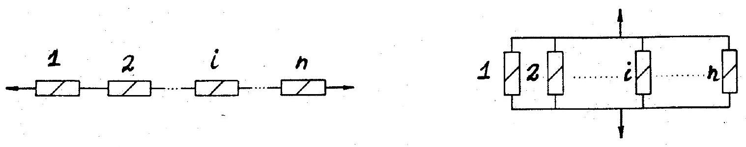
Fig. 10.1 Schematic representation of series and parallel systems#
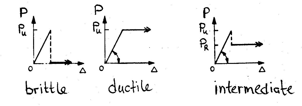
Fig. 10.2 Idealised load-displacement response of structural elements#
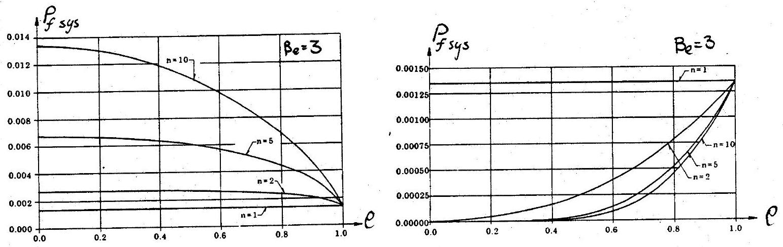
Fig. 10.3 Effect of element correlation and system size on failure probability (a) series system (b) parallel system#
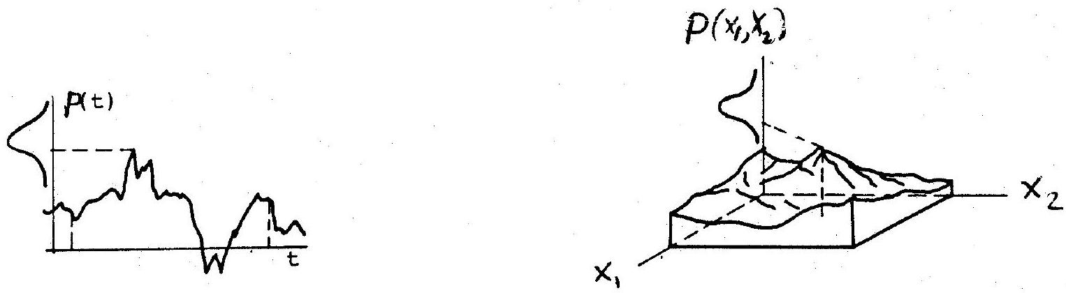
Fig. 10.4 Schematic representations (a) random process (b) random field#
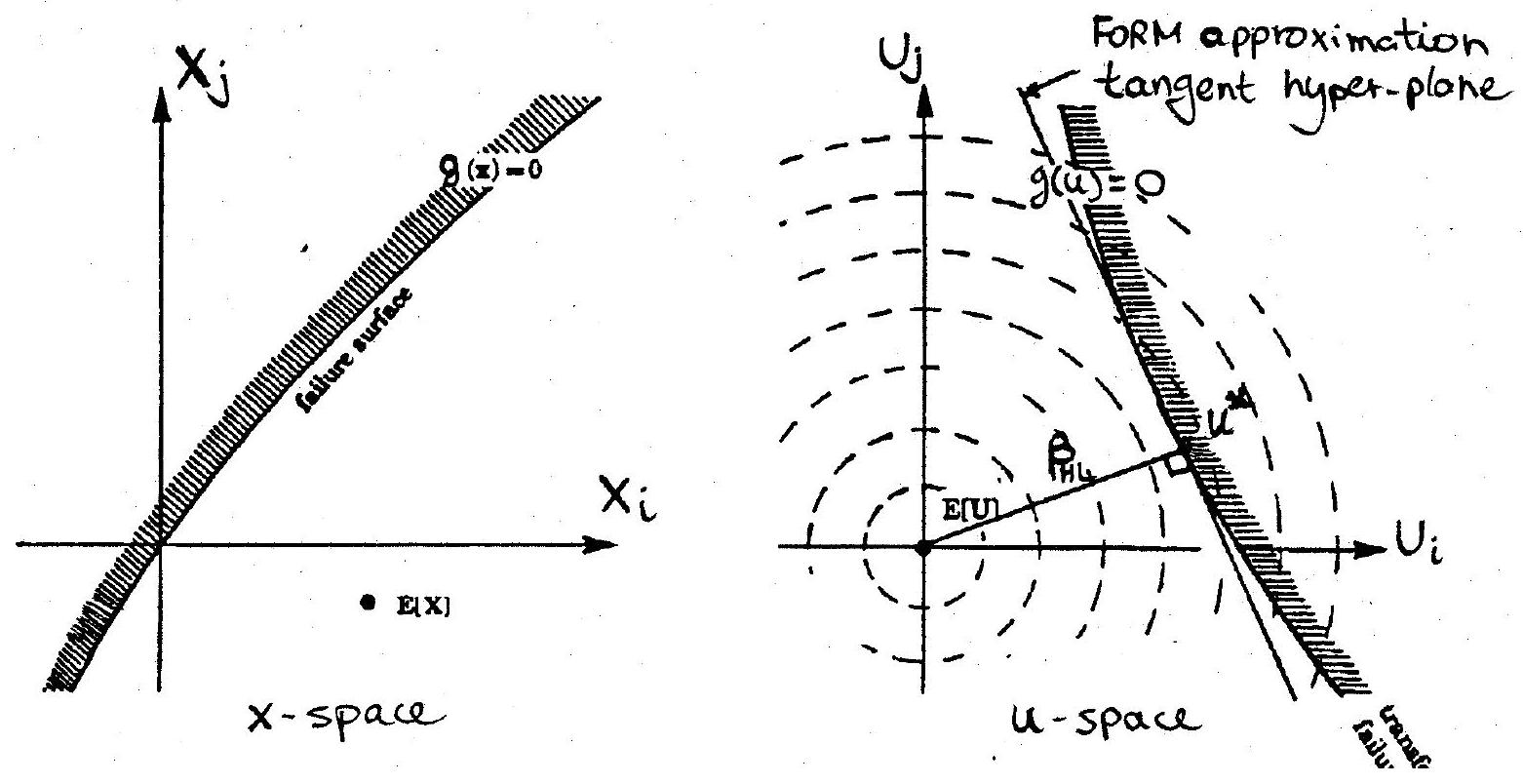
Fig. 10.5 Limit state surface in basic variable and standard normal space#
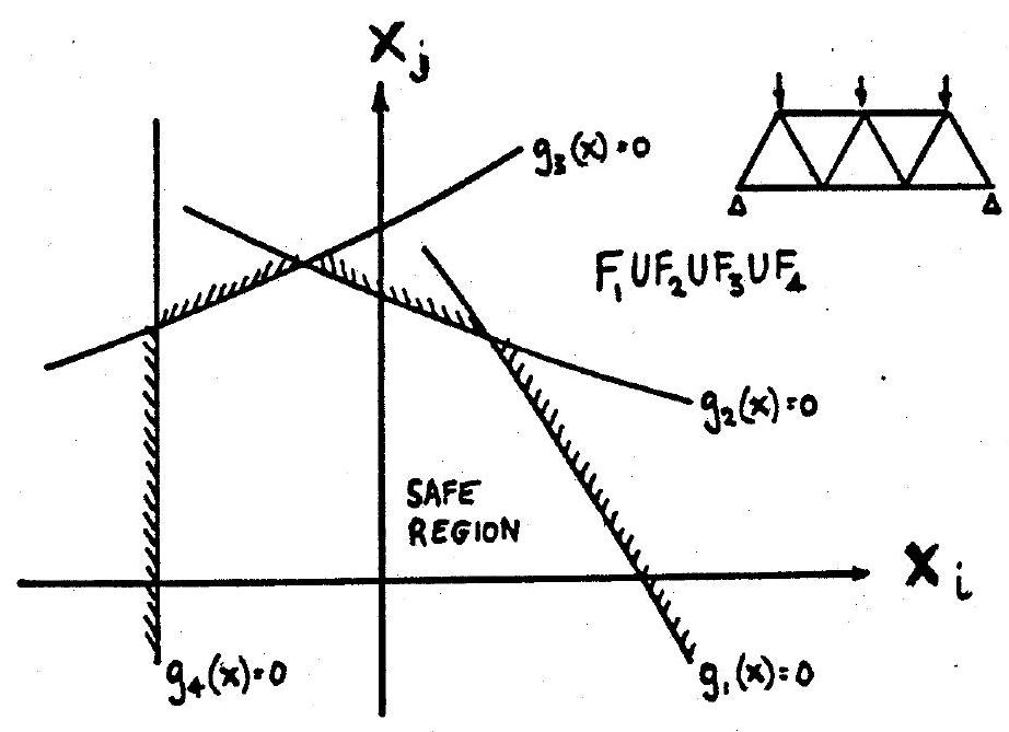
Fig. 10.6 Failure region as union of component failure events for series system#
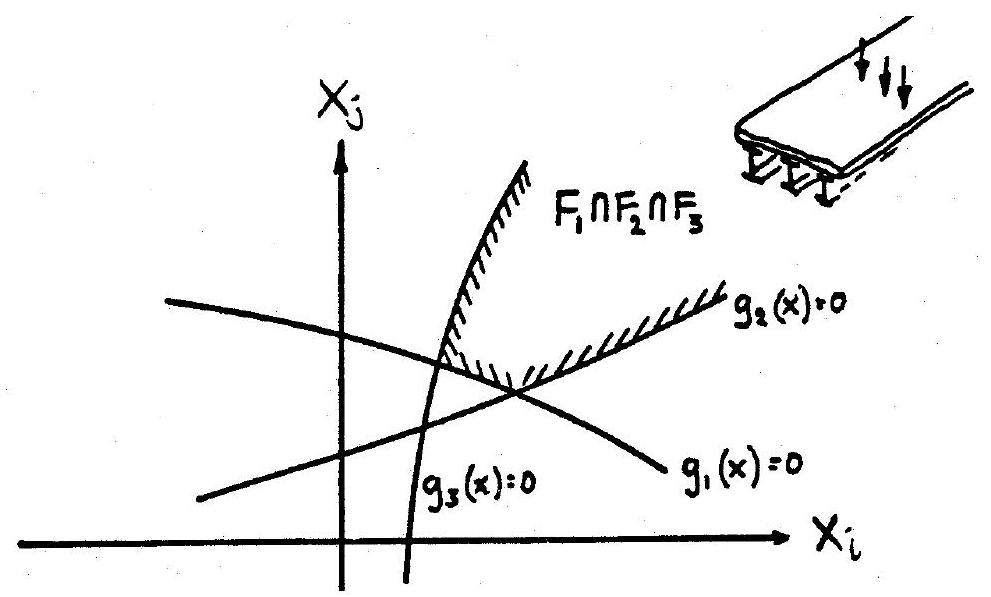
Fig. 10.7 Failure region as intersection of component failure events for parallel system#
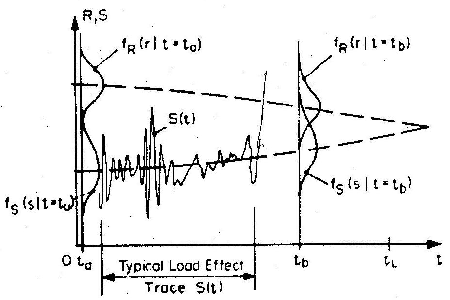
Fig. 10.8 General time-dependent reliability problem#
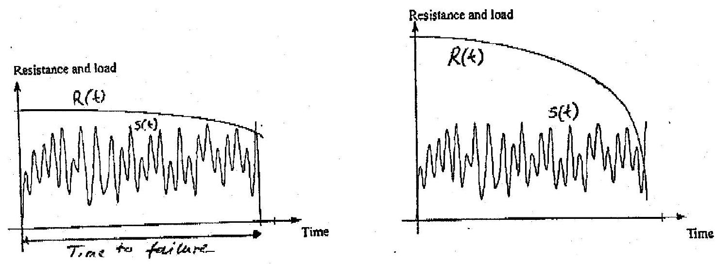
Fig. 10.9 Schematic representation of crossing problems (a) slowly varying resistance (b) rapidly varying resistance#
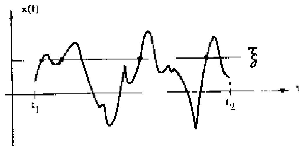
Fig. 10.10 Fundamental barrier crossing problem#
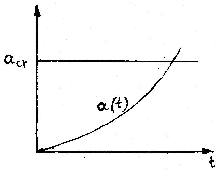
Fig. 10.11 Damage accumulation problem#
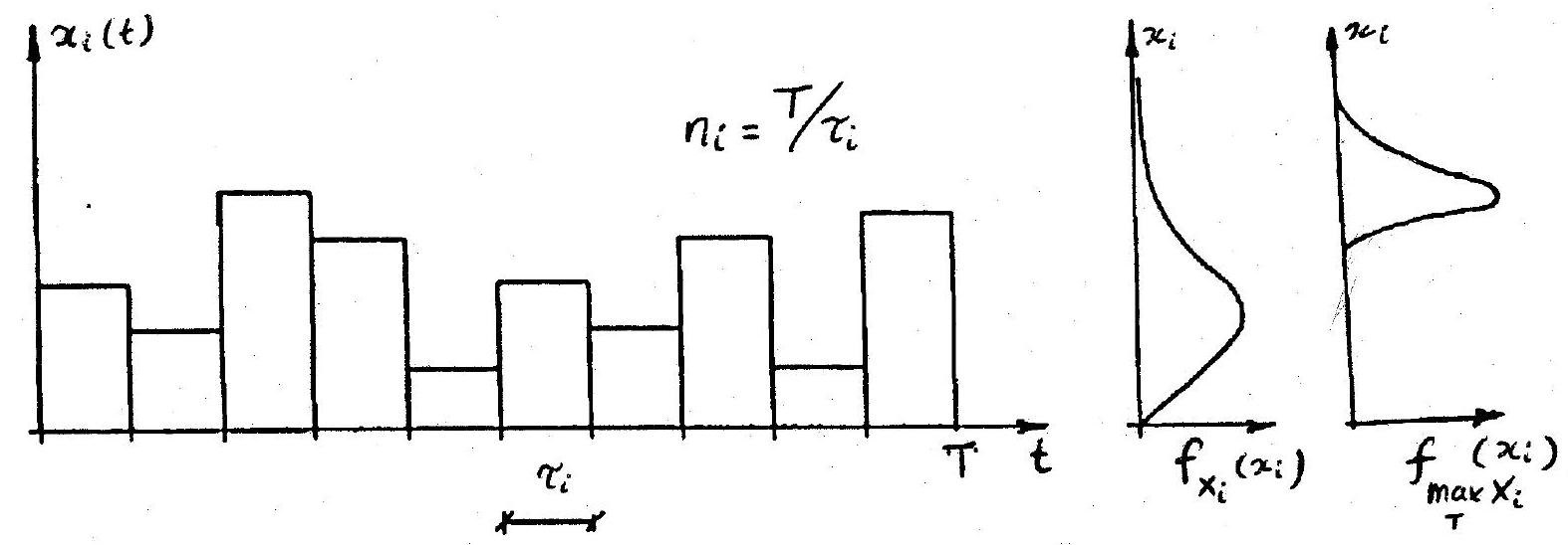
Fig. 10.12 Realization of an FBC process#
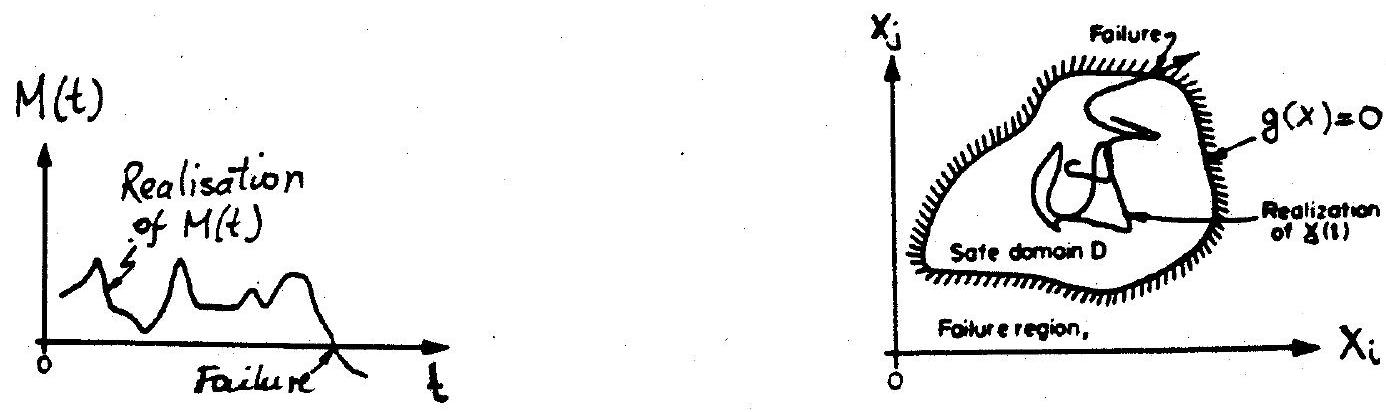
Fig. 10.13 Time-dependent safety margin and schematic representation of vector outcrossing#
10.7. Bibliography#
[C1] Ang A H S and Tang W H, Probability Concepts in Engineering Planning and Design, Vol. I & II, John Wiley, 1984.
[C2] Augusti G, Baratta A and Casciati F, Probabilistic Methods in Structural Engineering, Chapman and Hall, 1984.
[C3] Benjamin J R and Cornell C A, Probability, Statistics and Decision for Civil Engineers, McGraw Hill, 1970.
[C4] Bolotin V V, Statistical Methods in Structural Mechanics, Holden-Day, 1969.
[C5] Borges J F and Castanheta M, Structural Safety, Laboratorio Nacional de Engenharia Civil, Lisboa, 1985.
[C6] Ditlevsen O, Uncertainty Modelling, McGraw Hill, 1981.
[C7] Ditlevsen O and Madsen H O, Structural Reliability Methods, J Wiley, 1996.
[C8] Madsen H O, Krenk S and Lind N C, Methods of Structural Safety, Prentice-Hall, 1986.
[C9] Melchers R E, Structural Reliability: Analysis and Prediction, 2nd edition, J Wiley, 1999.
[C10] Thoft-Christensen P and Baker M J, Structural Reliability Theory and its Applications, Springer-Verlag, 1982.
[C11] Thoft-Christensen P and Murotsu Y, Application of Structural Systems Reliability Theory, Springer-Verlag, 1986.
[C12] CEB, First Order Concepts for Design Codes, CEB Bulletin No. 112, 1976.
[C13] CEB, Common Unified Rules for Different Types of Construction and Materials, Vol. 1, CEB Bulletin No. 116, 1976.
[C14] Construction Industry Research and Information Association (CIRIA), Rationalisation of Safety and Serviceability Factors in Structural Codes, Report 63, London, 1977.
[C15] International Organization for Standardization (ISO), General Principles on Reliability for Structures, ISO 2394, Third edition.