18. Thermal Actions

List of symbols:

\(\begin{array}{ll}A &= \text { cross-sectional area of the structural member}\\ C &= \text { coefficient for atmospheric clearness}\\ D &= \text { the intensity of diffused solar radiation}\\ I_y &= \text { main moment of inertia, direction of axis} y\\ I_z &= \text { main moment of inertia, direction of axis} z\\ Q &= \text { the intensity of total radiation}\\ S &= \text { the intensity of direct solar radiation}\\ T &= \text { temperature} \\ T_0 &= \text { initial temperature when structural member is restrained}\\ T_E &= \text { residual no-linear self-equilibrated component}\\ T_N &= \text { uniform temperature component} \\ \Delta T_N &= \text { range of uniform bridge temperature component} \\ \Delta T_M &= \text { linear temperature difference component} \\ \Delta T_{M,\text{heat}} &= \text { linear temperature difference component (heating)} \\ \Delta T_{M,\text{cool}} &= \text { linear temperature difference component (cooling)} \\ T_s &= \text { temperature of the bridge surface} \\ T_v &= \text { temperature of surrounding environment} \\ T_{eq} &= \text { equivalent temperature} \\ c &= \text { specific heat capacity} \\ h &= \text { altitude of sun}\\ h_c &= s\text { urface transfer coefficient} \\ k_s &= \text { absorption factor}\\ m &= \text { mean; number of optical masses of the atmosphere}\\ n &= \text { number of measurements}\\ s &= \text { standard deviation} \\ q &= \text { heat energy}\\ q_s &= \text { heat due to solar radiation}\\ q_r &= \text { heat due to re-radiation}\\ q_c &= \text { heat due to thermal transfer}\\ t &= \text { time} \\ \alpha &= \text { coefficient of linear expansion}\\ \alpha_e &= \text { exchange factor}\\ \gamma &= \text { hour angle of the sun} \\ \delta &= \text { angle of the sun declination}\\ \varepsilon &= \text { coefficient of emissivity; strain}\\ \lambda &= \text { heat conduction coefficient}\\ \rho &= \text { mass density}\\ \sigma &= \text { the Stephan-Boltzmann constant }\\ \varphi &= \text { geographical latitude of the locality}\end{array}\)

Conversion of units for temperatures considering °C, K and °F

°C = K – 273,15

°F = °C×1,8 + 32

18.1. Introduction

The structure exposed to climatic temperatures and operating process temperatures is subjected to non-stationary and spatially non-linear temperature fields causing strains or stresses. The same general principles may be applied for specification of temperatures and thermal effects on various types of construction works like buildings, industrial structures and bridges.

18.2. Basic Models For Temperature Effects In Structures

18.2.1. Basic variables

The basic variables influencing effects of thermal actions on structures include climatic agents, operating process temperatures, characteristics of construction works, geographical location of site, properties of atmosphere and terrain. Random properties of these variables may significantly affect the probabilistic structural analysis. Following aspects should be considered when analysing thermal effects on structures:

climatic characteristics

• shade air temperature (daily and seasonal changes)

• solar radiation (direct and diffused)

• wind speed (influenced by regional wind climate of the specific country and local factors as terrain roughness or orography in the location of the structure),

operating process temperature

• inner environment of the structure depending on its function,

characteristics of construction works

• space orientation of the structure (direction and height over the terrain)

• shape of the structure, dimensions and cross-sectional geometry

• joints of the structure, types of materials and used colours

• structural system

• thermal properties of materials (heat transfer coefficient at the surfaces, coefficient of absorptivity, coefficient of emissivity, specific heat, density, coefficient of linear expansion)

• other parameters such as moisture content, thickness of surfacing, building cladding

• initial temperature at which the structure is restrained,

properties of atmosphere and terrain

• emissivity of the atmosphere and terrain, location near some water source.

18.2.2. Mechanism of temperature development in the structure

The thermal exchange between the structure and its environment is influenced by three basic factors which may appear simultaneously

• the solar radiation and irradiation

• thermal convection

• thermal conduction.

In general, the heat flow process is a three-dimensional phenomenon. For structures having one dominating dimension such as bridges or beams, the variation of temperatures in the direction of the longitudinal axis is not usually significant and may be assumed constant along the length of a structure [18.01]. In these cases the temperature distribution can be considered as two-dimensional.

In many cases the transversal direction of temperature effects may also be neglected and one dimensional problem might be considered only in the direction of structural height (thickness).

For the solution of heat conduction problems in a structure, the Fourier heat conduction differential equation may be applied

(18.1)\[\frac{\partial T(z, t)}{\partial t}=\frac{\lambda}{c \rho} \frac{\partial^{2} T}{\partial z^{2}}\]

where \(t\) is the time, \(T\) is the temperature, \(c\) is the specific heat capacity of material, \(\rho\) is the mass density and \(\lambda\) is the heat conduction coefficient of material [18.02, 18.03]!. It should be noted that in some cases the properties of several materials may need to be considered. Recommended ranges of some thermophysical coefficients can be found in e.g. [18.04, 18.05]!. Some parameters may be considered as random variables represented by their probabilistic distribution functions.

Equation (18.1) is solved for the initial condition \(T=T_{0}\) in time \(t=t_{0}\) and boundary conditions on top and bottom structural surface with respect to the type of heat transmission between two adjacent mediums (surrounding environment and structure). The boundary conditions may be expressed as

(18.2)\[\frac{\lambda}{c \rho} \frac{\partial T}{\partial z} \eta_{z}+q=0\]

where \(\eta_{z}\) is the directional cosine of the normal vector and \(q\) is the heat energy exchange between the structure and its surrounding.

The heat energy \(q\) is composed of

(18.3)\[q=q_{s}+q_{r}+q_{c}\]

where \(q_{s}\) represents the heat due to solar radiation (direct and diffused), \(q_{r}\) the re-radiation and \(q_{c}\) the thermal transfer.

The heat due to solar radiation is given as

(18.4)\[q_{s}=k_{s} m Q\]

where \(k_{s}\) is the coefficient of surface absorptivity, \(m\) is the parameter dependent on cloudiness and \(Q\) is the intensity of total solar radiation (see Clause 18.3).

The re-radiation may be expressed as

(18.5)\[q_{r}=\varepsilon \sigma\left(T_{s}^{4}-T_{v}^{4}\right)\]

where \(\varepsilon\) is the bridge surface emissivity (in a range from 0,85 to 0,98 ), \(\sigma\) is Stephan Boltzmann constant \(\left(5,67 \times 10^{-8} W^{-2} ~K^{-4}\right), T_{s}\) is the temperature of the bridge surface and \(T_{v}\) is the temperature of surrounding environment.

The heat transfer due to conduction and convection is expressed as

(18.6)\[q_{c}=h_{c}\left(T_{s}-T_{v}\right)\]

where \(h_{c}\) is the surface transfer coefficient depending on the wind velocity.

For example the top surface heat transfer coefficient \(h_{s, t}\) includes both the radiation and convection losses (and gains) from the structural surface. The values of the coefficient \(h_{s, t}\) for concrete vary from \(14 Wm^{-2} ~K^{-1}\) to \(57 Wm^{-2} ~K^{-1}\) according to the exposure of the surface and the wind speed. For common exposure (considered \(`3^{\text {rd }}\) to \(5^{\text {th }}\) storeys of buildings in the interior of towns) and a wind speed of \(2,2 ~m / s\) to \(3,1 ~m / s\), the value of \(h_{s, t}\) is \(23 Wm^{-2} ~K^{-1}\). For the same exposure and a wind speed of almost zero, the value of \(h_{s, t}\) is \(19 Wm^{-2} ~K^{-1}\) [18.06].

18.2.3. Components of thermal actions

The temperature \(T(z, t)\) for a considered one dimensional problem of a structural member with the cross-sectional area \(A\), the centroid with principal axis of inertia \(y\) in the transversal direction and axis \(z\) in the direction of cross-sectional height may be decomposed to three temperature components on the basis of the following expression

(18.7)\[T(z, t)=T_{N}(z, t)+z \Delta T_{M z}(z, t)+T_{E}(z, t)\]

where \(T_{N}\) denotes the uniform temperature component (effective bridge temperature), \(\Delta T_{M z}\) the temperature difference component and \(T_{E}\) the residual non-linear self-equilibrated component.

The temperature components may be determined on the basis of integration of equation (18.7) across the area \(A\)

(18.8)\[\int_{A} T(z, t) d A=T_{N}(t) \int_{A} d A+\Delta T_{M z}(t) \int_{A} z d A+\int_{A} T_{E}(z, t) d A\]

where \(\int_{A} d A=A\), and \(\int_{A} z d A=0\) for the principal axis of inertia. It is considered \(\int_{A} T_{E}(z, t) d A=0\) for the self-equilibrated temperature component. The equation (18.8) may be rewritten under these assumptions as

(18.9)\[\int_{A} T(z, t) d A=T_{N}(t) A\]

and the uniform temperature component may be expressed as

(18.10)\[T_{N}(z, t)=\frac{1}{A} \int_{A} T(z, t) d A\]

Similarly the temperature difference component may be derived on the basis of the multiplication of equation (18.7) by variable \(z\) and its integration across the cross-sectional area \(A\) given as

(18.11)\[\Delta T_{M z}(z, t)=\frac{1}{I_{y}} \int_{A} T(z, t) z d A\]

where \(I_{y}\) is the main moment of inertia of a member cross-section with respect to the principal axis \(y\) of the cross-section and where the requirement \(\int_{A} T_{E}(z, t) z d A=0\) is considered.

The non-equilibrated component is expressed from equation (18.7) as

(18.12)\[T_(z, t)=T(z, t)-\left[T_{N}(t)+z \Delta T_{M z}(t)\right]\]

and for equations (18.10) and (18.11)

(18.13)\[T_{E}(z, t)=T(z, t)-\left[\frac{1}{A} \int_{A} T(z, t) d A+\frac{1}{I_{y}} \int_{A} T(z, t) z d A\right]\]

Presently all temperature components \(T_{N}, \Delta T_{M z}\) and \(T_{E}\) are based on temperature \(T(t, z)\) which was previously solved in equation (18.1).

18.2.4. Deformation and stress effects

The uniform temperature component leads to the longitudinal movements of a structure. In case the structure is restrained, tensile or compressive stresses should be taken into account.

The temperature difference components lead to the cross-sectional curvatures, in case that the structure is restrained they evoke moments.

The residual non-linear self-equilibrated component leads to the deplanation of structure and in case of its restrain to self-equilibrated stresses.

The temperature induced strains and therefore any resulting stresses, are dependent on the geometry and boundary conditions of the structural member being considered and on the physical properties of the material used.

18.3. Probabilistic models for radiation and temperature

Development of temperatures in a structure may be obtained either theoretically by means of the heat conduction method or experimentally by measuring the temperatures in many points of relevant structure with adequate frequency. A reliable theoretical prediction of the temperature fields in a structure is a quite difficult problem because it needs the integration of the Fourier heat conduction equation on a generally complex shaped domain under appropriate initial conditions, and with non-linear and time-dependent boundary conditions.

An important factor is the initial temperature of the structure in the relevant stage of its restraint [18.01, 18.07, 18.08]! which should be measured and recorded.

18.3.1. Shade air temperature

Shade air temperature has considerable effect on uniform temperature component [18.01, 18.08]! being mainly influenced by

• the daily and seasonal changes,

• the location of the site (altitude above the sea level, configuration of terrain)

• the wind velocity.

Information on the shade air temperature may be obtained from the National Meteorological Institute. The confidence on statistical evaluation of air parameters is dependent on the duration of observation. For statistical analysis of these parameters, the observation data for not less than 25 years should be applied [18.01, 18.08]!. However, different values of shade air temperature can be obtained by measuring in the location of site, dependent on specific local climatic conditions, e.g. frost pockets, where the difference can be more than 5°C. The extreme value probabilistic distributions may be applied for modelling the extremes of shade air temperature.

18.3.2. Uniform bridge temperature component

The uniform bridge temperature component may be specified on the basis of shade air temperatures and expression (18.10). For modelling the uniform temperature component, the extreme value probabilistic distribution may be applied. The uniform temperature component is commonly based on the three-day maxima of shade air temperature for concrete bridges and on one-day maxima for steel and composite bridges.

The skewness of the uniform bridge temperature component determined from experimental bridge measurements [18.01] is considerably less (between 0,2 to 0,6 ) than the skewness of the Gumbel distribution which is commonly recommended in prescriptive documents [18.08]. Therefore, the Weibull distribution may be preferably applied for the bridge uniform temperature component. However, the disadvantage of the Weibull distribution is its upper bound which is rather difficult to be estimated. More convenient seems to apply the skewness instead of trying to specify the upper bound of the distribution.

Three types of the extreme values distributions which may be applied for the probabilistic modelling of basic variables are illustrated in Fig. 18.1.

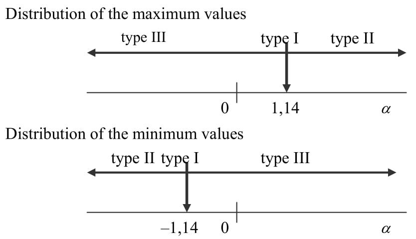
Fig. 18.1 Types of the extreme values distribution versus the skewness \(\alpha\)

The variation of the upper bound \(x_{\text {sup }}(m, s, a)\) with skewness \(a\) is illustrated in Fig. 18.2 for the mean temperature \(m\) from 30 to 36 °C and standard deviation \(s\) from 5 to 6 °C (with equal coefficient of variation 1/6).

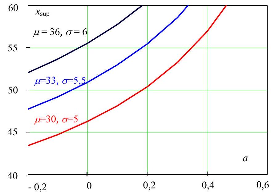
Fig. 18.2 Upper bound \(x_{\text {sup }}(m, s, a)\) of temperatures (in °C) versus skewness \(a\) for Weibull distribution

The document [18.01] introduces an estimated upper bound of extreme temperatures which is based on measurements of bridges in UK and Germany.

The upper bound of temperatures depends on the national climatic conditions of each country. It is influenced by number of days per year in which the extreme temperature may occur (a period of three months from June to August is considered). In some countries less or more days per year should be considered. The upper bound values in the document [18.01] may be not suitable for some other countries and should be based on statistically evaluated data.

The background document [18.01] gives several tables with statistically assessed parameters of uniform temperature component (mean, standard deviation and upper bound) of three-day maxima (Weibull maximum distribution) for concrete bridges, and one-day maxima for steel and composite bridges.

Statistical parameters of one-year maxima for uniform bridge temperature \(T_{N, \max }\) for steel and composite bridges are given in Table 18.1 based on the measurements of bridges in UK and Germany given in document [18.01].

Table 18.1 Statistical parameters of one-year maxima for uniform bridge temperature \(T_{N,max}\) for steel and composite bridges, in K (°C) (based on [1])

Bridge position and depth of surfacing	Mean in K (°C)	St. deviation
Steel bridge	313,15 (40)	2
Composite bridge	308,15 (35)	2

The mean values of uniform temperatures are slightly decreasing with increasing thickness of bridge surfacing while the value of standard deviation remains unchanged.

Statistical parameters of one-year maxima for expansion range of uniform bridge temperature component, \(\Delta T_{N, \text { exp }}\) for concrete bridges are given in Table 18.2 based on the measurements of bridges in UK and Germany given in document [18.01].

Table 18.2 Statistical parameters of one-year maxima for expansion range of uniform bridge temperature component, \(\Delta T_{N,exp}\) = \(T_{N,max}\) – 10°C for concrete bridges, in K (°C) (based on [1])

Depth [m]	Mean, in K (°C)	Standard deviation
	Box girder
2,0	296,15 (23)	2
4,7	295,15 (22)	2
	T girder
1,2	298,15 (25)	2
2,4	296,15 (23)	2
	Slab
0,6	297,15 (24)	2
1,2	294,15 (21)	2

To avoid possible inaccuracies from having a deterministic upper bound, local data may also be tuned to a three parameter lognormal distribution as it has no upper bound for positive skewness.

18.3.3. Solar radiation

Solar radiation has considerable influence on the temperature difference component and partly also on the uniform temperature component. The intensity of solar radiation depends on

• the geographical latitude of the site, on the clearness of the sky and the environment,

• the season,

• the orientation of the structural surface with respect to the sun,

• the colour and surface properties of the structure.

The observation data of solar radiation may be obtained from the National Meteorological Institute. The probabilistic model of solar radiation for the site location should be based on the statistical assessment of data.

When observation data are not available, an estimate of direct and diffused radiation can be obtained e.g. from ISO/TR 9492 [18.07]. The records of measurements of direct radiation \(S\) on the surface perpendicular to sun rays, diffused radiation \(D\) and total radiation \(Q\) are available in special reports of the Meteorological Institute, averaged for some time period (week, month).

Where observation data are not available, the intensity \(S_{m}\) of direct solar radiation under clear sky and non-varying clearness of atmosphere during the day may be approximately expressed as

(18.14)\[S_{m}=S_{0} /(1+C m)\]

where

\(S_{0}\) is the meteorological solar constant equal to \(1256 Wm^{-2}\),

\(C\) is the coefficient which depends on atmospheric clearness, for normal clearness it may be assumed as \(C=0,31\),

\(m\) is the number of optical masses of the atmosphere to be assumed according to the altitude of the sun \(h\), see Table 18.3.

Table 18.3 The optical masses \(m\) for the altitude of sun \(h\) [7])

Altitude of the sun \(h\), in degrees	Number of optical masses, \(m\)	Altitude of the sun \(h\), in degrees	Number of optical masses, \(m\)
90	1	16,4	3,5
41,7	1,5	14,3	4
30	2	12,6	4,5
23,5	2,5	11,3	5
19,3	3

The altitude of the sun above the horizon \(h\) may be determined as

(18.15)\[\sin h=\sin \varphi \sin \delta+\cos \varphi \cos \delta \cos \gamma\]

where

\(\varphi\) is the geographical latitude of the locality,

\(\delta\) is the angle of the sun declination,

\(\gamma\) is the hour angle of the sun, in degrees, \(\gamma=15 \tau\), where \(\tau\) is time in hours starting at noon.

The intensity of direct solar radiation on a horizontal surface is given as

(18.16)\[S^{\prime}=S \sin h\]

the intensity of diffused solar radiation on the horizontal surface is given as

(18.17)\[D=0,38~CS\]

and the intensity of total radiation on the horizontal surface is given as

(18.18)\[Q=S^{\prime}+D\]

Data on intensity of direct solar radiation on the surface normal to the sun rays can be used for evaluation of the intensity of radiation on vertical \(S_{v}\), and inclined surfaces of any orientation \(S_{\alpha}\) by the formulae

(18.19)\[S_{v}=S \cos \theta \]

(18.20)\[S_{\alpha}=S_{v} \sin \alpha+S^{\prime} \cos \alpha\]

where \(\theta\) is the angle between the direction of the sun ray and the normal to the surface at the given point of latitude \(\varphi\),

\(\alpha\) is the angle of inclination between the surface and the horizon.

The values of \(\cos \theta\) for surfaces of different orientation may be determined by the formulae

(18.21)\[\cos \theta_{S}=\cos \delta \sin \varphi \cos \gamma-\sin \delta \cos \varphi\]

(18.22)\[\cos \theta_{N}=\sin \delta \cos \varphi-\cos \delta \sin \varphi \cos \gamma\]

(18.23)\[\cos \theta_{E, W}=\cos \delta \sin \gamma\]

(18.24)\[\cos \theta_{NSE, SW}=\sqrt{ } 2 / 2(\cos \delta \sin \varphi \cos \gamma-\sin \delta \cos \varphi+\cos \delta \sin \gamma)\]

(18.25)\[\cos \theta_{NSE, NW}=\sqrt{ } 2 / 2(\cos \delta \sin \gamma+\sin \delta \cos \varphi-\cos \delta \sin \varphi \cos \gamma)\]

Using these formulae it may be calculated the intensity of direct solar radiation under a clear sky on the horizontal as well as vertical and inclined surfaces of different orientation for each hour of the day in any season corresponding to the latitude of the locality.

The intensity of diffused solar radiation on a vertical surface can be determined by an indirect method using the data of pyrheliometric observations for the diffused radiation of the horizontal surface and experimental data for the value of the relative illuminance of vertical surfaces of different orientation.

Due to a significant variety of influencing factors, an accurate description of the influence of the solar radiation on structure is complicated. Therefore, the equivalent temperature \(`T_{s}\) may be applied [18.07] for the assessment of solar radiation effects given as

(18.26)\[T_{s}=\frac{k_{s}}{\alpha_{e}} Q\]

where

\(Q\) is the intensity of the total (i.e. direct and diffused) solar radiation, \(Wm^{-2}\),

\(k_{s}\) is the absorption factor of solar radiation by the structure surface,

\(\alpha_{e}\) is the exchange factor as a result of convection and radiation, \(Wm^{-2} ~K^{-1}\).

The coefficient \(\alpha_{e}\) depends on the material and colour of the structure and on the wind velocity [18.03]. The equivalent temperature \(T_{s}\) is added during the structural analysis to the outdoor air temperatures. Both the daily distribution of \(T_{s}\) and the daily variation of outdoor air temperature can be expanded into Fourier series. The values of absorption factor \(k_{s}\) of solar radiation are given in Table 18.4.

Table 18.4 The absorption factor of solar radiation \(k_{s}\) by the structure surface

Material of structure	\(k_{s}\)
Asphalt	0,8 to 0,9
Clay brick	0,7 to 0,8
Concrete	0,6 to 0,7
Aluminium	0,4 to 0,5
Silica brick	0,3 to 0,4
Rendered, faced or coloured surfaces of materials and structures:
\(\quad\)- white and light grey	0,3 to 0,4
\(\quad\)- grey	0,4 to 0,5
\(\quad\)- red, brown, green	0,5 to 0,7
\(\quad\)- blue	0,7 to 0,8
\(\quad\)- dark-blue, black	0,8 to 0,9

The solar radiation is the leading variable for the temperature differences Here are multiple citations [18.01, 18.08]!. Information on short-wave solar radiation can be obtained from pyrheliometric observations, including direct radiation on the surface perpendicular to sun rays, diffused radiation and total radiation on the horizontal surfaces of the structure [18.07].

18.3.4. Difference bridge temperature component

For the determination of the vertical difference temperature component, the expression (18.11) should be solved taking into account the measurements of shade air temperatures and effects of solar radiation.

The statistical characteristics of the model of temperature difference component may be assessed on the basis of the extreme value probabilistic distribution. The skewness of the temperature difference component determined from the experimental measurements seems to be considerably less than the skewness of the Gumbel distribution. It appears that the Weibull or three parameter lognormal distributions may be preferably applied for modelling the temperature difference component.

Statistical parameters of one-year maxima for temperature differences \(\Delta T_{M \text {,heat }}\) (heating) for steel and composite bridges are given in Table 18.5 and for temperature differences \(\Delta T_{M, \text { cool }}\) (cooling) are given in Table 18.6 based on the measurements of bridges in UK and Germany given in the background document [18.01].

Table 18.5 Statistical parameters of one-year maxima of temperature differences \(\Delta T_{M,heat}\) for steel and composite bridges in K (°C) (based on [1])

Bridge	Mean in K (°C)	St. deviation
Steel	284,15 (11)	0,5
Composite	288,15 (15)	1

Table 18.6 Statistical parameters of one-year maxima of temperature difference \(\Delta T_{M,cool}\) in K (°C) for steel and composite bridges (based on [1])

Bridge	Mean in K (°C)	St. deviation
Steel	290,15 (17)	0,5
Composite	293,15 (20)	0,5

Statistical parameters of one-year maxima for temperature differences \(\Delta T_{M \text {,heat }}\) for concrete bridge are given in Table 18.7 based on the measurements of bridges in UK and Germany given in the document [18.01]. The mean of temperature difference is slightly decreasing with increasing thickness of the bridge surfacing while the value of standard deviation remains unchanged.

Table 18.7 Statistical parameters of one-year maxima of temperature differences \(\Delta T_{M,heat}\) in K (°C) for concrete bridges (based on [1])

Type	Depth [m]	Mean in K (°C)	St. deviation
Box girder	2,0	297,15 (24)	0,5
T-girder	1,2	288,15 (15)	1,5
slab	0,6	289,15 (16)	1,0

18.4. Action Effects

For the determination of action effects due to temperature components, the coefficient of linear expansion should be known.

18.4.1. Coefficients of linear expansion

Following relationship may be applied for determination of longitudinal displacements

(18.27)\[\varepsilon=\alpha T\]

where the coefficient of linear thermal expansion \(\alpha\) have influence on the resulting thermal effects. The coefficient \(\alpha\) changes partly systematically (due to the type of material) and partly randomly (due to the physical and chemical properties of material). For the determination of statistical characteristics of the coefficient \(\alpha\), it is necessary to evaluate data of the relevant material.

The coefficient \(\alpha\) for concrete may be expected in the range [18.09]

• concrete with common aggregate \(\alpha_{\min }=7 \times 10^{-6}\) to \(\alpha_{\max }=13 \times 10^{-6}\)

• concrete with lightweight aggregate \(\alpha_{\min }=5 \times 10^{-6}\) to \(\alpha_{\max }=11 \times 10^{-6}\)

depending on the type of cement, the composition of aggregate, on the humidity and the size of the structural cross-section. The humidity of material decreases with the increasing temperature of concrete influencing the value of coefficient \(\alpha\).

18.5. Model Uncertainities

Basic variables involved in the assessment of thermal actions on structures contain many uncertainties. Several factors influence the magnitude of resulting temperatures and their effects on structures including structural materials, their thermal properties, used colours, surfacing, geometry of a structure, its exposition to sun, shading by objects, air humidity, geographical and geomorphological position of site etc. It is also necessary to consider the accuracy of measurements (selected cross-sections, instrumentation), time period and procedure of evaluation. Daily temperatures (instantaneous part) and seasonal temperatures (long-term part) influence the thermal course within the structure.

For the assessment of the model uncertainty, it should be known model uncertainties of its individual variables. Some prior basic information concerning model uncertainties from other types of climatic actions (snow, wind) might be accepted.

The mean and coefficient of variation of the variables (for boundary conditions) entering the components of the heat energy \(q\) in eq. (18.3) may be expressed as

(18.28)\[E(q)=E\left(q_{s}\right)+E\left(q_{r}\right)+E\left(q_{c}\right) \]

(18.29)\[\sigma=\sqrt{\sigma\left(q_{s}\right)^{2}+\sigma\left(q_{r}\right)^{2}+\sigma\left(q_{c}\right)^{2}}\]

where uncorrelated variables are considered.

The model uncertainties of the basic variables for individual components of the heat energy \(q_{s}, q_{r}\) and \(q_{c}\) should also be considered.

The coefficients of variations of temperature components for several bridges based on the background document [18.01] and for measurements in three bridges in the Czech Republic (two prestressed concrete bridges and one composite steel concrete bridge [18.010]) are given in Annex A.

18.6. ANNEX A Probabilistic Models Based On Direct Bridge Measurements (examples from UK, Germany and Czech Republic)

18.6.1. Introduction

The basic information concerning the statistical characteristics of temperature components based on the measurements in several bridges in UK and Germany given in the background document [18.01] and in three bridges the Czech Republic given in the research report [18.010] are presented in Annex A. The type III maximum extreme value distribution is applied and the annual statistical parameters are specified in all presented cases.

The background document [18.01] includes information on five year measurements on steel and composite bridges (from 1981 to 1985) and on four year measurements on concrete bridge (1984-1988). The software Therm was also applied in [18.01] for specification of temperatures in various types of cross-sections in concrete bridges considering 10 year simulation of bridge temperatures.

The research report [18.010] gives measurements on D1 highway prestressed concrete box girder bridge in Koberovice (South-East part of Bohemia), on D8 highway prestressed concrete two beam bridge across river Ohre (West part of Bohemia) and composite steel concrete bridge across Slavici valley in Prague ring.

Additional information may be found in documents given in bibliography.

18.6.2. Uniform temperature component

18.6.2.1. Measurements of uniform temperature in bridges in UK and Germany

The one-year maxima of uniform bridge temperature component \(T_{N, \max }\) for steel bridges is given in Table 18.8 and for composite bridges in Table 18.9. The one-year maxima of uniform temperature ranges \(\Delta T_{N, \exp }\) for concrete bridges are given in Table 18.10. Table 18.8 to Table 18.10 gives information on selected bridges of the background document [18.01].

The model of uniform (effective) temperature component \(T_{N}\) may be based on the national isotherms of minimum and maximum shade air temperatures, or determined from evaluated data from the site location. The extreme value distribution may be applied.

Table 18.8 Statistical parameters of one-year maxima for uniform temperature \(T_{N,max}\) for steel bridge in K (°C) (web plate 20×4000 mm, bottom flange 600×40 mm, width of the bridge 15000 mm, length of cantilever 3000 mm)

Bridge position and depth of surfacing	Mean, in K (°C)	St. deviation	Skewness
North-south direction, east side of the cross-section, 50mm surfacing	313,25 (40,1)	1,1	-0,19
East-west direction, south side of the cross-section, 80mm surfacing	311,95 (38,8)	0,9	-0,30

Table 18.9 Statistical parameters of one-year maxima of uniform bridge temperature \(T_{N,max}\) for composite bridges in K (°C) (concrete slab 300 mm, web plate 20×400 mm, top flange 400×40, bottom flange 600×40 mm, width of bridge 15000 mm, length of cantilever 3000 mm)

Bridge position and depth of surfacing	Mean, in K (°C)	St. deviation	Skewness
North/south direction, east side of the cross-section, 50mm surfacing, coefficient \(\alpha=1,0 \times 10^{-5}\)	303,65 (30,5)	0,9	-0,16
North/south direction, east side of the cross-section, 50mm surfacing, coefficient \(\alpha=1,2 \times 10^{-5}\)	308,15 (35,0)	1,1	-0,14
East-west direction, south side cross- section, 80mm surfacing, \(\alpha=1,0 \times 10^{-5}\)	303,05 (29,9)	0,9	-0,12

Table 18.10 Statistical parameters of one-year maxima for expansion range of uniform bridge temperature component, \(T_{N,exp}\) = \(T_{N,max} – 10\)°C for concrete bridges, expressed in K and °C

Depth [m]	Mean, in K (°C)	Standard deviation	Skewness
	Box girder
2,0	296,35 (23,2)	2,1	0,44
3,3	295,85 (22,7)	2,0	0,49
4,7	295,05 (21,9)	2,0	0,53
	T girder
1,2	298,45 (25,3)	2,0	0,34
1,8	297,45 (24,3)	2,0	0,41
2,4	296,25 (23,1)	1,9	0,49
	Slab
0,6	296,65 (23,5)	2,1	0,40
0,9	294,75 (21,6)	2,1	0,52
1,2	293,65 (20,5)	2,0	0,58

18.6.2.2. Measurements of uniform temperature in the Czech Republic

One-year maxima of uniform bridge temperature component \(\Delta T_{N, \max }\) in the Koberovice bridge (prestressed concrete box girder, three spans \(54 ~m+74 ~m+54 ~m\), cross-section of \(4,2 ~m\), depth of surfacing \(0,12 ~m\)) are given in Table 18.11. The uniform bridge temperature is based on the one year maxima derived from 3-day extremes of temperatures (period from June to August, 1999 - 2002) which was obtained from averaged morning measurements of bridge in four points (in walls, in top and bottom sides) of the box girder.

Table 18.11 Statistical parameters of one-year maxima for uniform bridge temperature \(T_{N,max}\) for Koberovice bridge, in K (°C).

Mean, in K (°C)	Standard deviation	Skewness
298,45 (25,3)	1,1	-0,04

NOTE The characteristic value of uniform temperature component obtained on the basis of measurements in Koberovice bridge is compared with the characteristic value of uniform temperature component given in EN 1991-1-5 [18.08]. The characteristic value of uniform temperature component based on measurements in Koberovice bridge (see Table 18.11) is specified as

\[T_{N k, \max }=37,5^{\circ} C\]

The characteristic value of uniform temperature component based on EN 1991-1-5 [18.08] and Czech national map of isotherms is given as

\(T_{Nk, \max , EN}=T_{Nk, EN}+1,5^{\circ} C=38+1,5=39,5^{\circ} C \quad\) (for lower bound of isotherms \(T_{Nk, \max }=36+1,5=\) \(\left.37,5^{\circ} C\right)\)

It could be noted that obtained characteristic values of the uniform temperature component are in a good agreement.

One-year maxima of uniform bridge temperature component \(\Delta T_{N, \max }\) in the Doksany 11 span prestressed concrete two beam bridge in Highway D8 (across river Ohre, 2011-2013) are given in Table 18.12.

Table 18.12 Statistical parameters of one-year maxima of temperature difference component \(T_{N,heat}\) for Doksany prestressed concrete bridge, in K (°C)

Mean, in K (°C)	St. deviation	Skewness
295,45 (22,3)	2,5	0,6

One-year maxima of uniform bridge temperature component \(\Delta T_{N, \max }\) for the three span composite steel concrete Slavici bridge in Prague ring (close to exit of Lochkov tunnel, 2011-2013), are given in Table 18.13.

Table 18.13 Statistical parameters of one-year maxima of uniform temperature range \(T_{N,heat}\) for the composite steel concrete Slavici bridge, in K (°C)

Mean, in K (°C)	St. deviation	Skewness
299,95 (26,8)	3,3	0,55

18.6.2.3. Relationship between shade air temperature and uniform temperature component

The relationship between the extreme shade air temperature and uniform temperature component for the three types of bridge superstructure is recommended in EN 1991-1-5 [18.08].

Note: The maximum uniform temperature component \(T_{N, \max }\) and minimum uniform temperature component \(T_{N, \text { min }}\) considered in [18.08] for three types of bridges (in °C ) can be expressed as

\[\begin{split}\left. \begin{array}{ll} \text{Type 1,} & T_{N, \max} = T_{\max} + 16^\circ C \\ \text{Type 2,} & T_{N, \max} = T_{\max} + 4.5^\circ C \\ \text{Type 3,} & T_{N, \max} = T_{\max} + 1.5^\circ C \end{array} \right\} \text{for } 30^\circ C \leq T_{\max} \leq 50^\circ C \left. \begin{array}{ll} T_{N, \text { min }}=T_{\text {min }}-3^{\circ} C \\ T_{N, \text { min }}=T_{\text {min }}+4,5^{\circ} C \\ T_{N, \text { min }}=T_{\text {min }}+8^{\circ} C \end{array} \right\} \text { for }-50^{\circ} C \leq T_{\text {min }} \leq 0^{\circ} C\end{split}\]

based on the daily range of 10°C. For other daily ranges of temperature, the adjustment of temperature components \(T_{N, \max }\) and \(T_{N, \min }\) is indicated in the following Table based on the Background document [18.01].

Adjustment of the uniform temperature component for temperature daily ranges, in °C

Type of bridge deck	\(T_{N, \max }\)	\(T_{N, \text { min }}\)
1. Steel	\(T_{N, \max }+\left(10-\Delta_{2}\right) / 3\)	\(T_{N, \min }\)
2. Composite deck	\(T_{N, \max }+\left(10-\Delta_{2}\right) / 2\)	\(T_{N, \min }+\left(\Delta_{1}-10\right) / 2\)
3. Concrete deck	\(T_{N, \max }+\left(10-\Delta_{2}\right) / 2\)	\(T_{N, \text { min }}+\left(\Delta_{1}-10\right) / 4\)

\(\Delta_{1}\), resp. \(\Delta_{2}\) is the shade air temperature range for minimum, resp. maximum temperature conditions appropriate to the site location

18.6.3. Temperature difference components

18.6.3.1. Measurements of temperature difference component in bridges in UK and Germany

The results of statistical analysis of temperature differences \(\Delta T_{M z}\) for steel bridges based on one-year maxima (type III maximum value distribution) are indicated in Table 18.14 and Table 18.15, for composite bridges in Table 18.16 and Table 18.17, and for concrete bridges in Table 18.18 based on the document [18.01].

Table A.3.1 Statistical parameters of one-year maxima of temperature differences \(\Delta T_{M, \text { heat }}\) for steel bridges (top warmer than bottom), in \(\mathrm{K}\left({ }^{\circ} \mathrm{C}\right)\)

Table 18.14 Statistical parameters of one-year maxima of temperature differences \(T_{M,heat}\) for steel bridges (top warmer than bottom), in K (°C)

Bridge position and depth of surfacing	Mean, in K (°C)	St. deviation	Skewness
North/south direction, east side of the cross-section, 50 mm surfacing	283,95 (10,8)	0,4	-0,08
North/south direction, east side of the cross-section, 80 mm surfacing	281,75 (8,6)	0,4	-0,19
East-west direction, south side of the cross-section, 80 mm surfacing	281,85 (8,7)	0,4	-0,19

Table 18.15 Statistical parameters of one-year maxima of temperature differences \(T_{M,cool}\) for steel bridges (bottom warmer than top), in K (°C)

Bridge position, depth of surfacing and coefficient \(\alpha\)	Mean, in K (°C)	St. deviation	Skewness
North/south direction, east side of the cross-section, 50mm surfacing	288,55 (15,4)	0,5	-0,14
North/south direction, east side of the cross-section, 80mm surfacing	289,95 (16,8)	0,5	-0,30

Table 18.16 Statistical parameters of one-year maxima of temperature difference \(T_{M,heat}\) in K (°C) for composite bridges (top warmer than bottom)

Bridge position, depth of surfacing and coefficient \(\alpha\)	Mean, in K (°C)	St. deviation	Skewness
North/south direction, east side of the cross-section, 50 mm surfacing, \(\alpha=1,0 \times 10^{-5}\)	283,95 (10,8)	1,1	0,54
North/south direction, east side of the cross-section, 50 mm surfacing, \(\alpha=1,2 \times 10^{-5}\)	288,15 (15,0)	0,8	0,15
North/south or East/west directions, east side of the cross-section, 80mm surfacing, \(\alpha=1,0 \times 10^{-5}\)	282,85 (9,7)	0,4	-0,14

Table 18.17 Statistical parameters of one-year maxima of temperature difference \(T_{M,cool}\) in K (°C) for composite bridges (bottom warmer than top)

Bridge position, depth of surfacing and coefficient \(\alpha\)	Mean, in K (°C)	St. deviation	Skewness
North/South direction, east side of the cross-section, 50mm surfacing, \(\alpha=1,0 \times 10^{-5}\)	292,85 (19,7)	0,5	-0,28
North/south direction, east side of the cross-section, 50mm surfacing, \(\alpha=1,2 \times 10^{-5}\)	290,15 (17,0)	1,0	0,18
North/south direction, east side of the cross-section, 80mm surfacing, \(\alpha=1,0 \times 10^{-5}\)	292,85 (19,7)	0,6	-0,27
East-west direction, south side of the cross-section, 80mm surfacing, \(\alpha=\) \(1,0 \times 10^{-5}\)	289,15 (16,7)	1,0	0,13

Table 18.18 Statistical parameters of one-year maxima of temperature differences \(T_{M,heat}\) in K (°C) for concrete bridges.

Depth [m]	Mean, in °K (°C)	St. deviation	Skewness
	box girder
2,0	282,95 (9,8)	0,4	0,34
3,3	281,75 (8,6)	0,4	0,36
4,7	281,85 (8,7)	0,4	0,37
	T-girder
1,2	288,55 (15,4)	1,6	0,49
1,8	286,05 (12,9)	1,4	0,22
2,4	284,45 (11,3)	1,4	0,60
	slab
0,6	288,95 (15,8)	1,2	0,25
0,9	285,25 (12,1)	0,9	0,23
1,2	282,55 (9,4)	0,8	0,29

18.6.3.2. Measurements of temperature difference component in the Czech Republic

The results of measurements of temperature differences in the Koberovice bridge (concrete box girders, cross-section A of left bridge, cross-section D of right bridge) are shown in Table 18.19 and Table 18.20. The temperature differences are based on the 3 day extremes of the concrete box girder (measured in top and bottom of the box girder). The statistical characteristics for annual extremes of type III are given in Table 18.19 and Table 18.20.

Table 18.19 Statistical parameters of one-year maxima of temperature differences \(T_{M,heat}\) for Koberovice bridge, concrete box girder A, in K (°C)

Mean, in K (°C)	St. deviation	Skewness
281,35(8,2)	1,2	0,95

NOTE The characteristic value of temperature difference component obtained on the basis of measurements in Koberovice bridge is compared with the characteristic value of temperature difference component given in EN 1991-1-5 [18.08].

The characteristic value of temperature difference component based on measurements in Koberovice bridge is specified as

\[\Delta T_{M , \text { heat }}=10,75^{\circ} \]

The characteristic value of temperature difference component based on EN 1991-1-5 [18.08] is given as

\[\Delta T_{M , \text { heat,EN }}=12,5-2,5=10^{\circ} \]

It could be noted that obtained characteristic values of the temperature difference component are in a good agreement.

The results of three year measurements of Doksany bridge on Highway D8 (across river Ohre) are given for temperature difference component in Table 18.20 (2011-2013).

Table 18.20 Statistical parameters of one-year maxima of temperature difference component \(T_{M,heat}\) for Doksany prestressed concrete bridge, in K (°C)

Mean, in K (°C)	St. deviation	Skewness
279,55(6,4)	1,1	0,1

Results of three year measurements of Slavici composite steel concrete bridge in Prague ring is given for temperature difference component in Table 18.21 (2011-2013).

Table 18.21 Statistical parameters of one-year maxima of temperature difference component \(T_{M,heat}\) for Slavici composite steel concrete bridge, in K (°C)

Mean in K (°C)	St. deviation	Skewness
277,05(3,9)	0,6	0,6

18.6.4. Solar radiation for Koberovice bridge

The daily solar radiation was measured in the Meteorological station in Košetice (about \(12 ~km\) from the Koberovice bridge in the Czech Republic) from June to August 1999 -2001 (No. of observations \(n=276\)). Statistical parameters of daily global solar radiation and its components are given in Table 18.22.

Table 18.22 Statistical parameters of global solar radiation and its components (diffused and direct) from June to August 1999-2001 provided by the Meteorological station Košetice, in kJ/m2.

Statistical parameters	Global radiation	Diffused radiation	Direct radiation
Minimum	1832	1832	0
Maximum	29837	14342	25704
Mean	17696	8852,7	8802,9
Stand. deviation	6577	2622,8	7150,5
Coef. of variation	0,37	0,296	0,81
Skewness	-0,22	-0,46	0,52

The one-year maxima of global solar radiation is assessed on the basis of 3-day maxima based on the measurements provided by Meteorological station Košetice from June to August 1999 - 2001. The statistical parameters are indicated in {numref}`table-Statistical-parameters-of-one-year-maxima-for-global-solar-radiation-and-its-components-from-the-station-Košetice.

Table 18.23 Statistical parameters of one-year maxima for global solar radiation and its components (diffused and direct) from the station Košetice, in kJ/m2.

Statistical parameters	Global radiation	Diffused radiation	Direct radiation
Mean	30790	13620	17290
Standard deviation	1479	370	672
Coef. of variation	0,05	0,03	0,04
Skewness	-0,16	-0,55	-0,05
Upper limit	34890	14370	19370

For the global solar radiation and its components, the type III extreme value distribution may be applied.

The daily total and diffused solar radiation from June to August 2002 is illustrated in Fig. 18.3.

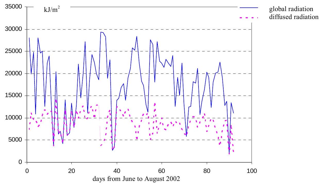
Fig. 18.3 The daily total and diffused solar radiation from June to August 2002 based on information from Meteorological Institute near Koberovice bridge

The daily course of measured temperatures in the Koberovice concrete box girder (left and right walls, top and bottom, outside temperatures (out) and inside temperatures (in) of the box girder) from 01/07 to 10/07/2002 is for illustration shown in Fig. 18.4.

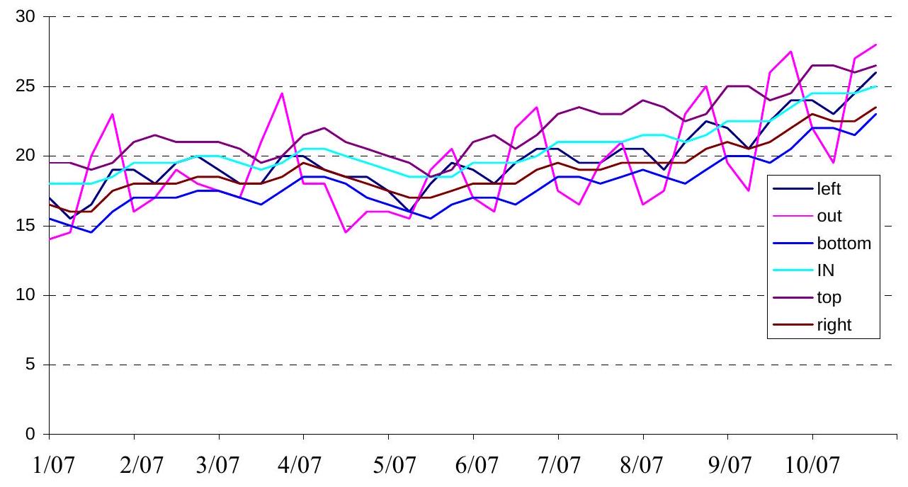
Fig. 18.4 The daily course of measured temperatures in the Koberovice concrete box girder in °C (left and right walls, top and bottom slabs, outside and inside temperatures) from 01/07 to 10 / 07 / 2002.

References

[18.01] (1,2,3,4,5,6,7,8,9,10,11,12,13,14,15,16,17,18,19,20)

New european code for thermal actions. 1999. Background document.

[18.02]

E. Mirambell and A. Aguado. Modelo de obtencion de distribuciones de temperaturas y de tensiones longitudinales autoequilibradas en puentes de hormigon. Revista internacional de métodos numéricos para cálculo y diseňo en ingeniería, 3(2):205–230, 1987.

[18.03] (1,2)

I. Mangerig. Klimatische temperaturbeansppruchung von stahl-und stahlverbund-brucken. Technical Report, Universitat Bochum, 1986.

[18.04]

I. Mangerig. Klimatische temperaturbeansppruchung von stahl-und stahlverbund-brucken. Technical Report, Universitat Bochum, 1986.

[18.05]

A.M. Neville. Properties of Concrete. Longman, London, 1986.

[18.06]

M. Emerson. The calculation of the distribution of temperature in bridges. Technical Report 561, TRRL Laboratory, Crowthorne, 1973.

[18.07] (1,2,3,4)

International Organization for Standardization. Iso/tr 9492: basis for design of structures – temperature climatic actions. Technical Report ISO/TR 9492, International Organization for Standardization, 1987.

[18.08] (1,2,3,4,5,6,7,8,9,10,11)

Eurocode 1: actions on structures - part 1-5: general actions – thermal actions. 2003.

[18.09]

Technical handbook 45. Actions on structures. Prague, 1987. Technical handbook 45.

[18.010] (1,2,3)

J. Markova, M. Holicky, and J. Kral. Optimisation of safety and working life of existing bridges. Research report, CTU in Prague Klokner Institute, 2013.

Additional References

1. Froli M., Barsotti R., Statistical analysis of thermal actions on a concrete segmental boxgirder bridge Structural Engineering International, 2000

2. TRRL Laboratory Report 696 Bridge temperatures estimated from shade temperatures, Crowthorne, 1976

3. TRRL Laboratory Report 748, W. Black et al., Bridge temperatures derived from measurement of movement, Crowthorne, 1976

4. TRRL Laboratory Report 783, M. Emerson, Temperatures in bridges during the hot summer of 1976, Crowthorne, 1977

5. TRRL Laboratory Report 641, J.D.Mortlock, The instrumentation of bridges for the measurement of temperature and movement, Crowthorne, 1974

6. White I.G., Non-linear differential temperature distributions in concrete bridge structures: a review of the current literature, Cement and concrete association, Technical report, 1979

7. Jones MR, Calculated deck plate temperatures for a steel box bridge, TRRL laboratory report, Crowthorne, 1977

8. TRRL Laboratory Report 783, M. Emerson, Extreme values bridge temperatures for design purposes, Crowthorne, 1996