
22. Fire#
List of symbols:
\(\begin{array}{ll}A_{f} &= \text { floor area}\\ A_{i} &= \text { area of the vertical opening i in the fire compartment} \left[m^{2}\right]\\ A_{t} &= \text { total internal surface area}\\ f &= \text { ventilation opening}\\ H_{i} &= \text { specific combustible energy for material}~i\\ m_{i} &= \text { derating factor between 0 and 1 , describing the degree of combustion}\\ M_{ki} &= \text { combustible mass present at} \Delta A \text { for material}~i\\ q_{o} &= \text { fire load density per unit floor area}\\ t &= \text { time}\\ t_{eq} &= \text { equivalent time of fire duration}\\ \alpha &= \text { parameter}\\ \beta_{f} &= \text { coefficient (model uncertainty)}\\ \theta &= \text { temperature in the compartment}\\ \theta_{0} &= \text { temperature at the start of the fire}\\ \theta_{A} &= \text { parameter}\end{array}\)
22.1. Fire ignition model#
The probability of a fire starting in a given building or area is modelled as a Poisson process with constant occurrence rate:
The occurrence rate \(v_{fire}\) can be written as a summation of local values over the floor area:
where \(\lambda(x, y)\) corresponds to the probability of fire ignition per year per \(m^{2}\) for a given occupancy type; \(A_{f}\) is the floor area of the fire compartment. As in most applications \(\lambda(x, y)\) can be simplied as a constant, and (22.2) can be simplified to:
Values for \(\lambda\) are presented in Table 22.1.
Type of building |
\(\lambda\) [m\(^{-2}\) year\(^{-1}\)] |
|---|---|
dwelling/school |
0.5 to 4 * 10\(^{-6}\) |
shop/office |
1 to * 10\(^{-6}\) |
industrial building |
2 to 10 * 10\(^{-6}\) |
22.2. Flashover occurrence#
After ignition there are various ways in which a fire can develop. The fire might extinguish itself after a certain period of time because no other combustible material is present. The fire may be detected very early and be extinguished by hand. An automatic sprinkler system may operate or the fire brigade may arrive in time to prevent flash over. Only in a minority of cases does a fire develop into a fully developed room or compartment fire; sometimes the fire may break through a barrier and start a fire in another compartment. From the structural point of view only these fully developed or post flashover fires (see Fig. 22.1) may lead to failure. For very large fire compartments having a very large concentration of fire loads, e.g. industrial buildings, a local fire of high intensity also may lead to (localised) structural damage.
The occurrence rate of flashover is given by:
The probability of a flashover once a fire has taken place, can obviously be influenced by the presence of sprinklers and fire brigades. Numerical values for the analysis are presented in Table 22.2.
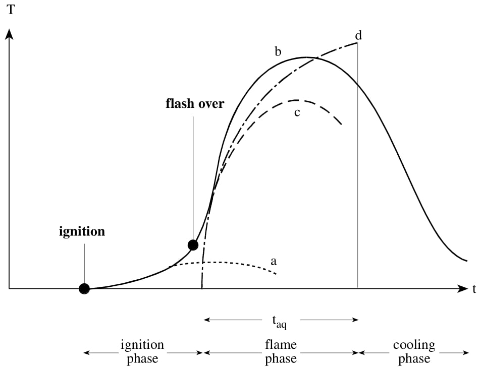
Fig. 22.1 Schematic presentation of a temperature-time curve#
Curve (a) represents the temperature-time curve when a sprinkler system or a timely fire brigade action is successful.
Curve (b) presents the temperature-time relation for a fully developed fire.
Curve (c) indicates the limited influence of a fire brigade arriving after flashover has taken place.
Curve (d) indicates the ISO-standard temperature curve (see section 19.4.2.).
Protection method |
P {flashover \(\mid\) ignition} |
|---|---|
Public fire brigade |
10\(^{-1}\) |
Sprinkler |
10\(^{-2}\) |
High standard fire brigade on site, combined with alarm system (industries only) |
10\(^{-3}\) to 10\(^{-2}\) |
Both sprinkler and high standard residential fire brigade |
10\(^{-4}\) |
22.3. Combustible material modelling#
The available combustible material can be considered as a random field, which in general might be nonhomogeneous as well as nonstationary. The intensity of the field \(q\) at some point in space and time is defined as:
\(m_{i}=\) derating factor between 0 and 1 , describing the degree of combustion
\(M_{ki}=\) combustible mass present at \(A_{f}\) for material \(i\)
\(H_{i}\) = specific combustible energy for material \(i\)
\(A_{f}=\) considered floor area
In some cases the intensity \(q\) may also depend on a vertical ordinate.
The non-dimensional factor \(\mu_{i}\) is a function of the fuel type, the geometrical properties of the fuel, and the position of the fuel in the fire compartment, among other things. For some types of fire load components, \(m_{i}\) depends on the time of fire duration and on the gas temperature-time characteristics of the compartment fire. Probabilistic models for \(q\) are presented in Table 22.3.
Type of fire compartment |
Mean value |
Coefficient of variation |
|---|---|---|
1: Dwellings |
500 |
0.20 |
2: Offices |
600 |
0.30 |
3: Schools |
350 |
0.20 |
4: Hospitals |
450 |
0.30 |
5: Hotels |
300 |
0.25 |
22.4. Temperature-time relationship#
22.4.1. Scientific models#
For known characteristics of both the combustible material and the compartment, the post flash over period of the temperature time curve can be calculated from energy and mass balance equations.
Many variables can be introduced as random in the model, for instance:
the amount and spatial distributions of combustible material;
the effective energy value;
the rate of combustion;
the ventilation characteristics;
air use and gas production parameters;
thermal conductivity properties;
model uncertainties.
In addition, the development of the fire may depend on events like collapse of windows or containments, which may change the ventilation conditions or the available amount of combustible material respectively.
As a simplification the following assumptions may be used.
the combustible material is wood;
the wood is spread uniformly over the floor area;
the fire compartment is of a standard building material (brick, concrete);
the fire is controlled by ventilation and not by the amount of fuel load (this is conservative);
the initial temperature is 20\(^{\circ} c\).
In this case the temperature time curve depends on two parameters:
the floor averaged fire load density \(q_{o}\);
the opening factor \(f\).
The opening factor \(f\) is defined as:
where:
\(A_{t}=\) total internal surface area of the fire compartment, i.e. the area of the walls, floor and ceiling, including the openings \(\left[m^{2}\right]\)
\(A_{i}=\) area of the vertical opening \(i\) in the fire compartment \(\left[m^{2}\right]\)
\(h_{i}\) value of the height of opening \(i[m]\)
For a fire compartment which also contains horizontal openings, the opening factor can be calculated from a similar expression. In calculating the opening factor, it is assumed that ordinary window glass is immediately destroyed when fire breaks out.
In many cases it will be possible to indicate a physical maximum \(f_{\max }\). The actual value of \(f\) in a fire should be modelled as a random quantity according to:
\(\zeta=\) random parameter (see Table 22.4)
To avoid negative values of \(f\), this lognormal distribution should be cut off at \(\zeta=1\). In addition one should multiply the resulting temperatures by an overall model uncertainty factor \(\theta_{\text {model }}\).
22.4.2. Engineering models#
In many engineering applications, use is made of equivalent standard temperature-time-relationship according to ISO 834:
with:
\(\theta=\) temperature in the compartment
\(\theta_{o}=\) temperature at the start of the fire
\(\theta_{A}=\) parameter
\(\alpha=\) parameter
\(t=\) time
\(t_{eq}=\) equivalent time of fire duration
\(\beta_{f}=\) coefficient (model uncertainty)
\(q_{o}=\) fire load density per unit floor area
\(A_{f}=\) floor area
\(A_{t}=\) total internal surface area
\(f=\) ventilation opening (see (22.6), (22.7))
Numerical values and probabilistic models are given in Table 22.4.
Variable |
Distribution |
Mean |
Standard deviation |
|---|---|---|---|
\(\zeta\) |
truncated lognormal \(^{1)}\) |
0.2 |
0.2 |
\(\beta_{f}\) |
lognormal |
4.0 sm\(^{2.25}\)/MJ |
1.0 |
\(\theta_{o}\) |
deterministic |
20\(^{\circ}\)c |
- |
\(\theta_{A}\) |
deterministic |
345 K |
- |
\(\alpha\) |
deterministic |
0.13 s\(^{-1}\) |
- |
\({ }^{1)}\) values of \(\zeta>1\) should be supressed