29. Soil Properties

Symbols used

\(\begin{array}{ll}\underline{a} \quad & \text { vector of average trend coefficients } \\ \underline{\hat{a}} \quad & \text { estimator of } \underline{a} \\ b \quad & \text { field correlation parameter } \\ C_{f}(\Delta \underline{x}) \quad & \text { auto covariance function } \\ \cos () \quad & \text { cosine function } \\ \operatorname{cov}() \quad & \text { covariance } \\ \operatorname{COV}() \quad & \text { covariance matrix } \\ D \quad & \text { field correlation parameter } \\ \underline{D} \quad & \text { vector of field correlation parameters } \\ \operatorname{det}() \quad & \text { determinant of a matrix } \\ E[~] \quad & \text { expected mean value } \\ \exp () \quad & \text { exponent function } \\ F() \quad & \text { polynomial shape function } \\ \underline{F}() \quad & \text { vector of polynomial shape functions } \\ f_{p}() \quad & \text { zero mean fluctuation field of (soil) property } p \\ I() \quad & \text { integral / average } \\ I_{0}(), J_{0}() \quad & \text { Bessel functions } ( 1^{\text {st }} \text { kind, order zero) } \\ L, L_{j} \quad & \text { dimension (length), directional dimension } \\ L_{f}() \quad & \text { likelihood function } \\ m_{p}() \quad & \text { average trend of (soil) property } p\\ P[e] \quad & \text { probability of some event } e \\ P[F] \quad & \text { probability of failure } \\ P\left[e_{1} \mid e_{2}\right] \quad & \text { conditional probability of event } e_{1} \text { given event } e_{2} \\ P_{j} \quad & \text { observed value } \\ p d f^{\prime \prime}() \quad & \text { posterior probability density function } \\ p d f^{\prime}() \quad & \text { prior probability density function } \\ R \quad & \text { correlation matrix } \\ r() \quad & \text { auto correlation function } \\ S \quad & \text { surface or volume affected by geotechnical mechanism (generic) }\\ S_{j} \quad & \text { scenario of subsoil stratigraphy } \\ \tan () \quad & \text { tangent function } \\ \underline{x}=(x, y, z) \quad & \text { vector of spatial coordinates, horizontal: }~x~\text{and}~y ;~\text{vertical} ~z\\ \operatorname{var}() \quad & \text { variance } \\ \alpha \quad & \text { ratio of variances } \\ \alpha_{j} \quad & \text { correlation radius } \\ \gamma(\tau) \quad & \text { semivariogram; semivariance as function of separation distance } \\ \Gamma^{2}() \quad & \text { variance reduction factor } \\ \Delta \underline{x}=(\Delta x, \Delta y, \Delta z)^{T} \quad & \text { vector of separation distances (lag components) }\\ \delta \quad & \text { scale of fluctuation } \\ \delta_{j} \quad & \text { directional scale of fluctuation } \\ \delta_{e q} \quad & \text { equivalent scale of fluctuation } \\ \rho_{f}() \quad & \text { normalized auto covariance function (auto correlation function) } \\ \sigma \quad & \text { standard deviation of random variable or random field (generic) } \\ \sigma^{2} \quad & \text { variance of random variable or random field (generic) } \\ \sigma_{p}^{2} \quad & \text { variance of property } p \\ \sigma_{r p}{ }^{2} \quad & \text { variance of testing imperfections } \\ \tau \quad & \text { separation distance (lag) }\end{array}\)

29.1. Introduction

The term Soil Properties refers to a collection of characteristics of a soil body, which affect the response to loading or other actions. Soil properties include:

• soil stratigraphy, i.e. boundaries for subvolumes containing a single soil type - denoted as a soil unit in the following

• continuum properties, such as physical or mechanical parameters or state properties within each of the soil units, e.g. stiffness, compressibility, shear strength, permeability, overconsolidation ratio, initial pore pressures, etc.

Together with basic characteristics of behaviour of each soil unit, e.g. drained, undrained or partially drained behaviour, these items constitute the basic components of a soil model. Distinction of soil units is usually made on the basis of lithologal and geotechnical classification (sand, clay, organic material, or mixtures, compaction and consistency) and basic characteristics of response to loading.

Although reliability of foundations or other structures in soils is also controlled by uncertainties of applied loads and other construction materials (concrete or steel), a characteristic feature of geotechnical structures is the dominating role of the uncertainties of soil properties. This chapter focusses on probabilistic models to take these uncertainties of soil properties into account.

29.2. Uncertainties of Soil Properties

Various sources of uncertainty of soil properties may be distinguished:

• spatial variability of soil properties. Patterns of variability may be either continuous or discrete

• limited soil survey and laboratory or in situ testing

• inaccuracy of soil investigation methods and erroneous interpretation of investigation results.

Continuous spatial variability:

Continuum properties of a soil unit may vary continuously from one spot to another throughout the unit. The pattern of variability may be characterized by an average trend of variation, e.g. increase with depth, and continuous fluctuations around the average trend. This type of characterization also applies to continuously varying boundaries of soil units, e.g. depth level and thickness of a soil layer. Usually, this type of variability is modeled as a continuous stationary random field. In section 29.3. the basics of such models will be further outlined.

Parameters in a geotechnical analysis usually refer to averages of continuum properties over some surface area or some volume; e.g. average shear strength along a sliding surface or average stiffness of a volume affected by loading. Hence, relevant uncertainties of soil parameters in a geotechnical analysis concern usually uncertainties of its averages over affected surfaces of volumes. Random field modeling of “point to point” variations forms the basis for quantitative assessment of uncertainties of averaged soil parameters.

Discrete spatial variability:

Soil units with continuous spatial variability may be mixed with dislocations such as faults, lenses or fills, depending on the geological and morphologial history. Though local of nature, these phenomena may have a large effect on behaviour of structures built on or in the ground. Often exact locations and sizes of local phenomena are difficult to infer from, if at all revealed by, soil survey campaigns.

Limited soil survey and testing:

Information about subsurface conditions is acquired by field investigation in discrete survey points (tested samples from borings, SPT-records) or at discrete survey lines (CPT or geophysical records). Soil data is therefore generally only available for a small part of the relevant soil volume which implies, as a consequence, uncertainties which are somehow statistical of nature. Two types may be distinguished:

• inaccurate statistics of soil property distributions (continuum parameters and continuous soil layer boundaries)

• potential errors in the soil stratigraphy (e.g. missing local phenomena, anomalies).

Both types of uncertainties may be reduced at the expense of additional survey or testing. Considering continuous soil properties, the effect of additional survey and testing is the reduction of the error of estimated statistics by means of statistical sample theory or geostatistical approaches.

Considering potential errors of soil stratigraphy, the effect of additional survey is likely to be a reduction of the probability of occurrence of such errors. However, the process of assessment of soil stratigraphy from available soil data is for a significant part based on subjective engineering judgement. Hence, quantification of probabilities of stratigraphical errors, and its reduction due to additional survey, is also subject of engineering judgement. Probabilistic approaches to assess probabilities of occurrence of potential errors in the soil stratigraphy, related to type, extent and intensity of soil investigation, are far from well developed. Yet it seems that the effects of such errors can be more drastic than the effects of inaccurate statistics of continuous soil properties. In section 29.5., some hints will be provided concerning how to get along with this kind of uncertainties.

Inaccuracy of soil investigation method:

Inaccuracies may be caused by sample disturbance, test imperfections, such as poor reproducibility of tests or poor correlation between in situ test results and basic soil parameters, and human factors in conducting tests and interpretation of soil investigation results. Though this type of inaccuracies is often not the least important source of uncertainty, only part of it can be taken into account explicitly in probabilistic analyses. Gross errors of test equipment and in conducting tests must be avoided by appropriate quality assurance procedures. Gross errors in interpretation of soil investigation must be avoided by a thorough control scheme and an expert review.

29.3. Continuous Stochastic Models for Spatial Fluctuations

29.3.1. Concept of stationary random field modeling

Field representation

A random field is a conceivable model to characterize continuous spatial fluctuations of a soil property within a soil unit. In this concept, the actual value of a soil property at each location within the unit is assumed to be a realisation of a random variable. Usually, parameters of the random field model have to be determined from only one realisation. Therefore the random field model should satisfy certain ergodicity conditions at least locally.

Stationarity (or homogeneity) in a strict sense means that the entire joint probability density function (jpdf) of soil property values at an arbitrary number of locations within the soil unit is invariable under an arbitrary common translation of the locations. A more relaxed criterion is that expected mean value and variance of the soil property is constant throughout the soil unit and that the covariance of the soil property values at two locations is a function of the separation distance, or distance components, between the locations only. Random fields satisfying only the relaxed criteria are called stationary in a weak sense.

In the sequel only weak stationarity criteria will be considered. Normal (Gaussian) or log-normal random fields fulfilling the weak stationarity conditions are also stationary in a strict sense. For most soil properties the assumption of normality or log-normality is adequate.

A straightforward extension of the constant mean field model is that the expected mean value may vary, for example with depth, reflecting an average trend. The spatial model then reads:

(29.1)\[p(\underline{x})=m_{p}(\underline{x})+f_{p}(\underline{x})\]

where \(\underline{x}\) denotes a vector of spatial coordinates \(\underline{x}=(x, y, z)^{T}, p(\underline{x})\) the soil property value at location \(\underline{x}\), \(m_{p}(\underline{x})\) the average trend and \(f_{p}(\underline{x})\) a zero mean, (weakly) stationary, random field. Unless stated otherwise, in the sequel \(x\) and \(y\) will be considered horizontal coordinates and \(z\) the vertical one.

Usually the average trend function will be chosen as a linear composition of shape functions, for example low degree polynomials, and trend coefficients, i.e. \(m_{p}(\underline{x})=\underline{a}^{T} \underline{F}(z)\), where the transposed vector \(\underline{a}^{T}=\left(a_{1}, a_{2}, \ldots a_{m}\right)\) represents trend coefficients and \(\underline{F}(z)\) is a vector \(\left(F_{1}(z), F_{2}(z), \ldots F_{m}(z)\right)^{T}\) of polynomial shape functions of degree \(\leq(m-1)\).

More general, the average trend function may be a function of the location vector \(\underline{x}\), instead of the depth coordinate \(z\) only. In that case the polynomial shape functions change accordingly into \(F_{j}(\underline{x})\) \((j=1 \ldots m)\). Note that a constant mean field may be considered as a special case of a field with average trend and constant trend coefficients. In that case the trend coefficient vector is a simple scalar which is constant throughout the field and the corresponding shape function \(F_{1}(\underline{x})=1\). The concept of (weak) stationarity can be straightforwardly extended to fields with average trend. Such a field is (weakly) stationary when the trend coefficients are constant througout the field and the centered, i.e. zero mean, field of random fluctuations is (weakly) stationary.

A further extension concerns location dependency of the field variance. For example when the variance increases with depth, according to some specifically assumed pattern, the field representation changes into:

(29.2)\[p(\underline{x})=m_{p}(\underline{x})+s(z) f_{p}(\underline{x})\]

where the shape function \(s(z)\) reflects the pattern of change of the standard deviation with depth. In the sequel, this case will not be elaborated further.

Covariance structure of zero mean random field

Intensity and type of fluctuations of the zero mean field is characterized by its autocovariance function:

(29.3)\[C_{f_{p}}(\Delta \underline{x})=E\left[f_{p}(\underline{x}+\Delta \underline{x}) f_{p}(\underline{x})\right]\]

where \(\Delta \underline{x}=(\Delta x, \Delta y, \Delta z)^{T}\) is the vector of separation distances (“lag components”) and \(C_{f p}(\Delta \underline{x})\) the autocovariance function. Note that \(C_{f p}(0)=\sigma_{f p}^{2}\), the variance of the field. For real valued fields there is symmetry with respect to arguments, i.e. \(C_{f p}(\Delta x, \Delta y, \Delta z)=C_{f p}(|\Delta x|,|\Delta y|,|\Delta z|)\).

The function \(\rho_{f p}(\Delta\underline{x})=C_{f p}(\Delta \underline{x}) / \sigma_{f p}^{2}\) is called the normalized autocovariance function (autocorrelation function).

For field modeling purposes parameterized shape functions may be assumed to model the normalized autocovariance function. These shape functions should satisfy certain conditions in order to be admissible.

Some important modeling concepts regarding the autocovariance structure will be discussed briefly.

\(\underline{Separability}:\)

The autocovariance structure of a random field is called separable if the normalized autocovariance function can be written as a multiplication of normalized autocovariance functions for each of the field directions, i.e. \(\rho_{f p}(\Delta x, \Delta y, \Delta z)=\rho_{f p ; x}(\Delta x)~\rho_{f p ; y}(\Delta y)~\rho_{f p ; z}(\Delta z)\). The autocovariance structure may be partly separable, for example w.r.t. horizontal and vertical dimensions, i.e. \(\rho_{f p}(\Delta x, \Delta y, \Delta z)=\rho_{f p ; x y}(\Delta x, \Delta y)\) \(\rho_{f p ; z}(\Delta z)\).

Quite generally, if \(\rho_{1}\left(\Delta \underline{x}^{(m)}\right)\) and \(\rho_{2}\left(\Delta \underline{x}^{(k)}\right)\) are admissible normalized autocovariance functions for an m and k-dimensional field respectively, then \(\rho_{3}\left(\Delta \underline{x}^{(m)}, \Delta \underline{x}^{(k)}\right)=\rho_{1}\left(\Delta \underline{x}^{(m)}\right) \rho_{2}\left(\Delta \underline{x}^{(k)}\right)\) is an admissible normalized autocovariance function for an (m+k)-dimensional field.

\(\underline{Isotropy}:\)

The autocovariance structure is called isotropic if the normalized autocovariance depends on the Euclidian distances between field points only, instead of the axis directional distance components, i.e . \(\rho_{f p}(\Delta x, \Delta y, \Delta z)=\rho_{f p ; i}\left(\left(\Delta x^{2}+\Delta y^{2}+\Delta z^{2}\right)^{1 / 2}\right)\). Also the autocovariance structure may be partly isotropical, for example w.r.t. horizontal field directions: \(\rho_{f p}(\Delta x, \Delta y, \Delta z)=\rho_{f p ; i}\left(\left(\Delta x^{2}+\Delta y^{2}\right)^{1 / 2}, \Delta z\right)\).
Isotropy implies that the autocovariance function is invariant to orthonormal transformation of the field coordinates.

\(\underline{Ergodicity}:\)

An important modeling concept regarding statistical inference of field statistics is ergodicity. Ergodicity implies stationarity. A random field is ergodic (in a wide sense) if every one of the statistical parameters can be inferred from one single realization of the field. Usually one is interested in not all, but only some of the field statistics. The ergodicity concept may then be defined with respect to these parameters. For example, ergodicity w.r.t. the expected mean value and ergodicity w.r.t. the autocovariance structure.

For ergodicity w.r.t. the mean (in case of constant mean fields) or ergodicity w.r.t. average trend coefficients (in case the average trend coefficients are constant throughout the field), this implies that the autocovariance function must tend to zero for large lag, however this condition is not sufficient.

\(\underline{Positive~definiteness}:\)

The variance of any finite linear combination of values at any locations in the field must always be positive. This condition leads to the requirement that the covariance function must be positive definite. Verifying the positive definiteness of a parameterized autocovariance function can be done using Fourier transforms, but the procedure is difficult, and so in practice this requirement is usually met by selecting the function from one of those listed below (all of which have been shown to be positive definite).

One dimensional fields

Table 29.1 shows some admissible types of (normalized) autocovariance functions, as suggested in geotechnical and geohydrological literature, in a one dimensional representation.

Table 29.1 Some admissible types of normalized autocovariance functions

Type	Normalized autocovariance function: \(\rho_{f p}(\tau)=C_{f p}(\tau) / C_{f p}(0)\)
1. Exponential	\(\exp \left(-\frac{|\tau|}{D}\right)\)
2. Exponential, oscillatory	\(\exp \left(-\frac{|\tau|}{D}\right) \cos (b \tau)\)
3. Quadratic exponential (Gaussian)	\(\exp \left(-\left(\frac{\tau}{D}\right)^{2}\right)\)
4 Quadratic exponential oscillatory	\(\exp \left(-\left(\frac{\tau}{D}\right)^{2}\right) J_{0}(b \tau)\)
5. Bilinear note: applicability restricted to 1-D fields	\(\left(1-\frac{\mid \tau \mid}{D}\right) \qquad \text{for} \mid \tau \mid \leq D\) \(0 \hspace{5.8em} \text{for} \mid \tau \mid > D\)

Remarks:
\(J_{0}(.)\) is Bessel function of first kind and order zero
\(D\) and \(b\) are correlation parameters

One dimensional random fields with normalized autocovariance functions of type 1,2 or 5 are “almost surely” (a.s.) continuous but not differentiable (i.e. non-smooth), random fields with a normalized autocovariance function which is twice differentiable at zero lag \((\tau=0)\) are a.s. differentiable (i.e. smooth).

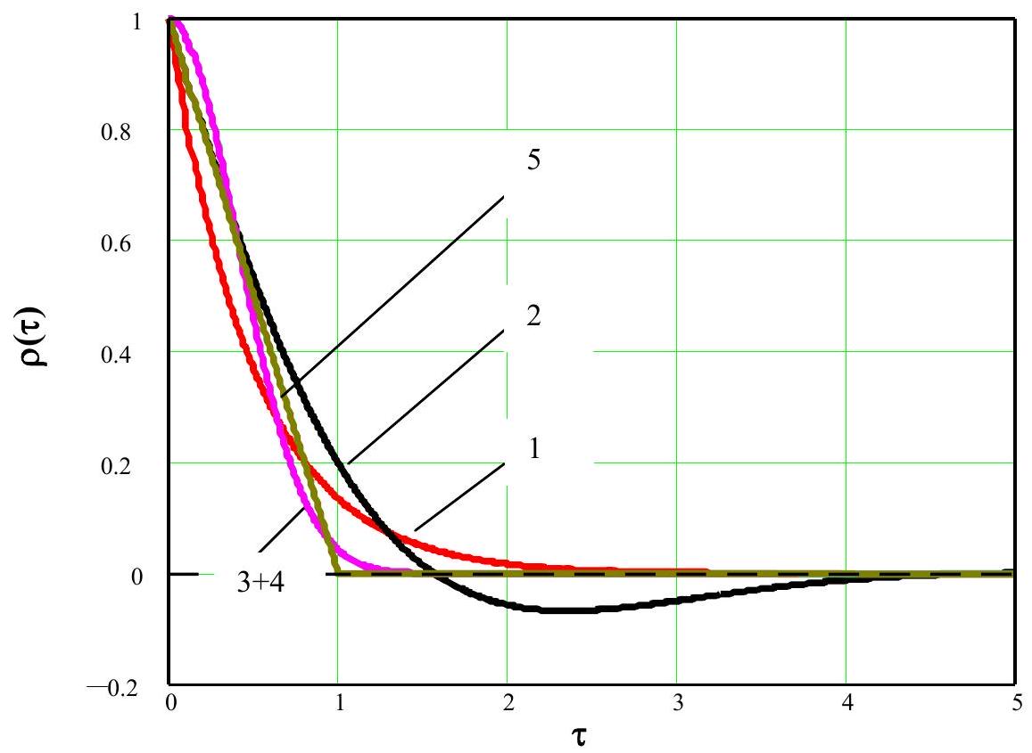
Fig. 29.1 Admissible normalized covariance functions of Table 29.1

2- and 3-dimensional fields

Based on the types in Table 29.1, admissible normalized autocovariance functions for 2- or 3-dimensional fields can be derived, e.g.:

\(\underline{Exponential}:\)

(29.4)\[\rho_{f_{p}}(\Delta x, \Delta y, \Delta z)=\exp \left(-\frac{|\Delta x|}{D_{x}}-\frac{|\Delta y|}{D_{y}}-\frac{|\Delta z|}{D_{z}}\right)\]

or in the case of horizontal isotropy:

(29.5)\[\rho_{f_{p}}(\Delta x, \Delta y, \Delta z)=\exp \left(-\frac{\sqrt{\Delta x^{2}+\Delta y^{2}}}{D_{h}}-\frac{|\Delta z|}{D_{z}}\right)\]

\(\underline{Gaussian}:\)

(29.6)\[\rho_{f_{p}}(\Delta x, \Delta y, \Delta z)=\exp \left(-\left(\frac{\Delta x}{D_{x}}\right)^{2}-\left(\frac{\Delta y}{D_{y}}\right)^{2}-\left(\frac{\Delta z}{D_{z}}\right)^{2}\right)\]

or in the case of horizontal isotropy:

(29.7)\[\rho_{f_{p}}(\Delta x, \Delta y, \Delta z)=\exp \left(-\left(\frac{\sqrt{\Delta x^{2}+\Delta y^{2}}}{D_{h}}\right)^{2}-\left(\frac{\Delta z}{D_{z}}\right)^{2}\right)\]

Note that the Bilinear autocovariance function (Type 5 in Table 29.1) is not admissible for 2- and 3-dimensional fields, because it does not fulfil the positive-definiteness criterion.

29.3.2. Scale of fluctuation

The scale of fluctuation (or correlation radius) for a one dimensional real valued field is defined as, c.f. [29.01]:

(29.8)\[\delta=2 \int_{0}^{\infty} \rho_{f p}(\tau) d \tau\]

Table 29.2 shows the relation between the scale of fluctuation and the correlation parameters for the normalized covariance function types in Table 29.1.

Table 29.2 Scales of Fluctuation

Type	Scale of fluctuation \(\delta\)
1.	\(\delta=2 D\)
2.	\(\delta=\frac{2 D}{1+b^{2} D^{2}}\)
3.	\(\delta=D \sqrt{\pi}\)
4	\(\delta=D \sqrt{\pi} \exp \left(-\frac{1}{8} b^{2} D^{2}\right) I_{0}\left(\frac{1}{8} b^{2} D^{2}\right)\)
5.	\(\delta=D\)

Remarks:
\(I_{0}( )\) is Bessel function of first kind and order zero

More generally, the scale of fluctuation \(\delta\) is defined as the radius of an equivalent “unit step” normalized covariance function, i.e. \(\rho(\tau)=1\) for \(\tau \leq \delta\) and \(=0\) for \(\tau>\delta\), \(\tau\) being the Euclidian lag, which contains the same volume \(\alpha\) of correlation as the normalized covariance function for the \(\mathrm{n}(=1,2,3)\) dimensional field.

(29.9)\[\alpha_{n}=2^{n} \int_{0}^{\infty} \int_{0}^{\infty} \ldots \int_{0}^{\infty} \rho_{f_{p}}\left(\tau_{1}, \tau_{2}, \ldots \tau_{n}\right)~d \tau_{1}~d \tau_{2} \ldots . d \tau_{n}\]

where \(\mathrm{n}=1,2,3\). In case of a 2-dimensional field:

(29.10)\[\begin{split}\begin{aligned} & \alpha_{2}=2^{2} \int_{0}^{\infty} \int_{0}^{\infty} \rho_{f_{p}}\left(\tau_{1}, \tau_{2}\right) d \tau_{1}~d \tau_{2} \\ & \delta_{e q}=\sqrt{\frac{\alpha_{2}}{\pi}} \end{aligned}\end{split}\]

In case of a 2-dimensional isotropical field \(\left(\tau_{12}=\sqrt{ }\left(\tau_{I}^{2}+\tau_{2}^{2}\right) \right )\)

(29.11)\[\begin{split}\begin{aligned} & \alpha_{2}=2 \pi \int_{0}^{\infty} \tau_{12} \rho_{f_{p}}\left(\tau_{12}\right) d \tau_{12} \\ & \delta_{2}=\sqrt{\frac{\alpha_{2}}{\pi}} \end{aligned}\end{split}\]

and, analogously in the case of spherical isotropy : \(\tau_{123}=\sqrt{ }\left(\tau_{1}{ }^{2}+\tau_{2}{ }^{2}+\tau_{3}{ }^{2}\right)\) :

(29.12)\[\begin{split}\begin{aligned} & \alpha_{3}=2 \pi^{2} \int_{0}^{\infty} \tau_{123}^{2}~\rho_{f_{p}}\left(\tau_{123}\right) d \tau_{123} \\ & \delta_{3}=\sqrt[3]{\frac{3 \alpha_{3}}{4 \pi}} \end{aligned}\end{split}\]

The correlation radius can be interpreted as a scalar measure, reflecting the average spatial extension of the field where strong correlation is present.

Measurements of horizontal scales of fluctuation of shearing strength in fluvial clays range range from 60 up to 200m and more, whereas vertical scales of fluctuation in these soil types range from some decimeters up to some metres. Indications of horizontal scales of fluctuation of average cone resistance, based on CPT records in deep glacial sand, range from 40 to 80 m, whereas the vertical scale of fluctuation in these tests ranged from 0.5 to 0.8 m. Appendix 29.7.A gives an impression of scales of fluctuation of soil parameters, as derived from reported experimental data in literature.

29.3.3. Spatial averaging

Parameters in geotechnical analyses usually refer to averages of a soil property over a sliding surface or a rupture zone in an ultimate failure analysis or significantly strained volumes in a deformation analysis. If the dimensions of such surfaces or volumes exceed the scales of fluctuation of the soil property, spatial averaging of fluctuations is substantial. This implies that the variance of an averaged soil property over a sliding surface or affected vlume is likely to be substantially less than the field variance, which is mainly based on small sample tests (e.g. triaxial tests) or small affected volumes in insitu tests (e.g. CPT’s, vane tests etc.).

Consider a soil property, c.f. eq. (29.1), in which \(m_{p}(\underline{x})\) is a constant \(m_{p}\). Its average over a vertical plane surface ( \(x, z\)-plane) with height \(h\) and width \(b\) reads:

(29.13)\[I_{b h}(p)=\frac{1}{b h} \int_{0}^{b} \int_{0}^{h} p(\underline{x}) d x d z=\frac{1}{b h} \int_{0}^{b} \int_{0}^{h}\left(m_{p}+f_{p}(\underline{x})\right) d x d z\]

The mean expected value equals: \(E\left[I_{b h}\right]=m_{p}\), the variance of \(I_{b h}(p)\) reads:

(29.14)\[\begin{split}\begin{aligned} & \operatorname{var}\left(I_{b h}(p)\right)=\frac{1}{b^{2} h^{2}} \int_{0}^{b} \int_{0}^{b} \int_{0}^{h} \int_{0}^{h} E\left[f_{p}(x, z) f_{p}(\xi, \eta)\right] d x~d \xi~d z~ d \eta \\ \\ & =\frac{\sigma_{f_{p}}^{2}}{b^{2} h^{2}} \int_{0}^{b} \int_{0}^{b} \int_{0}^{h} \int_{0}^{h} \rho_{f_{p}}(x-\xi, z-\eta) d x~d \xi~d z~d \eta \\ \\ & =\frac{4 \sigma_{f_{p}}^{2}}{b h} \int_{0}^{b} \int_{0}^{h}\left(1-\frac{\tau_{1}}{b}\right)\left(1-\frac{\tau_{2}}{h}\right) \rho_{f_{p}}\left(\tau_{1}, \tau_{2}\right) d \tau_{1}~d \tau_{2} \\ \\ & =\sigma_{f_{p}}^{2} \Gamma^{2}(b, h) \end{aligned}\end{split}\]

where \(\tau_{1}=x-\xi, \tau_{2}=z-\eta\), and \(\Gamma^{2}(b, h)\) is referred to as variance reduction factor.

If the normalized covariance function one of the separable type then eq. (29.14) can be written as:

(29.15)\[\operatorname{var}\left(I_{b h}(p)\right)=\sigma_{f_{p}}^{2} \Gamma^{2}(b) \Gamma^{2}(h)\]

where \(\Gamma^{2}(b)\) and \(\Gamma^{2}(h)\) are variance reduction factors:

(29.16)\[\Gamma^{2}(b)=\frac{2}{b} \int_{0}^{b}\left(1-\frac{\tau}{b}\right) \rho_{f_{p}}(\tau) d \tau\]

For large \(b\) compared to the correlation radius \(\alpha_{l}\) equation (29.16) tends to:

(29.17)\[\Gamma^{2}(b) \approx \frac{\alpha_{1}}{b}\]

Similar expressions are valid for \(\Gamma^{2}(h)\). Fig. 29.2 shows variance reduction factors for the normalized covariance functions of Table 29.1.

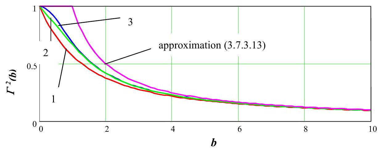
Fig. 29.2 Variance reduction factors for normalized covariance functions of Table 29.1

Realistic estimates of \(b / D_{h}\) for sliding surfaces in dike or road embankments range in the order of 0.5 to 2 , so variance reduction due to averaging in a horizontal direction may range between 0.95 to 0.4 . Realistic estimates of \(h / D_{v}\) for potential sliding modes in dike or road embankments on soft soil range from 5 and up. From Fig. 29.2 it can be seen that averaging in the vertical direction significantly reduces the variances of spatial fluctuations.

Quite generally the variance reduction factor for averaging in one, two or three dimensions may be approximated as:

(29.18)\[\begin{split}\begin{aligned} \Gamma^{2}\left(L_{1} \ldots L_{n}\right)=1 & \qquad \text { for }\left(L_{1} \ldots L_{n}\right) \leq \alpha_{n} \\ =\frac{\alpha_{n}}{\left(L_{1} \ldots L_{n}\right)} & \qquad \text { for } \left(L_{1} \ldots L_{n}\right)>\alpha_{n} \quad(n=1,2,3) \end{aligned}\end{split}\]

where \(L_{1}, L_{2}\) and \(L_{3}\) are the lengthes over which averaging takes place and \(\alpha_{1}, \alpha_{2}, \alpha_{3}\) are the correlation radii, as defined in eq. (29.9). In case of “separable” normalized autocovariance functions, i.e. which can be written as a multiplication of factors for each of the dimensions of a 2- or 3-D surface or volume, the total variance reduction factor can, for the 3-D case. be written as:

(29.19)\[\Gamma^{2}\left(L_{1} L_{2} L_{3}\right)=\Gamma^{2}\left(L_{1}\right) \Gamma^{2}\left(L_{2}\right) \Gamma^{2}\left(L_{3}\right)\]

Numerical approach

In general, averaging surfaces or volumes may not be parallel to the coordinate axes. A rough approach, as suggested by [29.01], is to assess the averaging dimensions by orthogonal projection of the averaging surface or volume at the coordinate axes, and proceed with the approximation (29.18) or (29.19) for the projected dimensions. This is a fairly good approach for averages over volumes. However, a more sophisticated approach is desirable for averages over surfaces (e.g. failure surfaces in limit state equilibrium analyses), as outlined by Rackwitz [29.02]. To that purpose surface integrals need to be computed. For example, assume that the surface \(S\) has the following parametric representation:

(29.20)\[S:\lbrace(x, y, z)\rbrace \quad \text { with } \quad z=h(x, y), \quad(x, y) \in B\]

where \(B\) is the projection of surface \(S\) onto the \((x, y)\)-plane. Then the average along surface \(S\) of some property \(p(\underline{x})=m_{p}+f_{p}(\underline{x})\), where \(f_{p}(\underline{x})\) is a zero mean homogeneous fluctuation field, reads:

(29.21)\[I_{S}(p)=\frac{1}{A(S)} \int_{S}\left(m_{p}+f_{p}(\underline{x})\right) d S(\underline{x})\]

where \(\mathrm{A}(S)\) is the area of the surface \(S\). The expected mean value \(E\left[I_{S}(p)\right]=m_{p}\) and the variance equals:

(29.22)\[\begin{split}\begin{aligned} & \operatorname{var}\left(I_{S}(p)\right)=\frac{\sigma_{f_{p}}^{2}}{A(S)^{2}} \int_{S(\underline{x})} \int_{S(\underline{\zeta})} \rho_{f_{p}}(\underline{x}-\underline{\zeta})~d S(\underline{x})~d S(\underline{\zeta}) \\ \\ & =\frac{\sigma_{f_{p}}^{2}}{A(S)^{2}} \int_{B(x, y)} \int_{ B(\eta, \xi)} \rho_{f_{p}}(x-\eta, y-\xi, h(x, y)-h(\eta, \xi)) \ldots \end{aligned} \\ \qquad \cdots \sqrt{1+\left(\frac{\partial h(x, y)}{\partial x}\right)^{2}+\left(\frac{\partial h(x, y)}{\partial y}\right)^{2}} \sqrt{1+\left(\frac{\partial h(\eta, \xi)}{\partial \eta}\right)^{2}+\left(\frac{\partial h(\eta, \xi)}{\partial \xi}\right)^{2}} d x~d y~d \eta~d \xi\end{split}\]

Covariances of averages of the soil property along different surfaces \(S_{j}\) and \(S_{k}\) can be expressed as:

(29.23)\[\begin{split}\begin{gathered} \operatorname{cov}\left(I_{S_{j}}(p), I_{S_{k}}(p)\right)=\frac{\sigma_{f_{p}}^{2}}{A\left(S_{j}\right) A\left(S_{k}\right)} \int_{B_{j}(x, y)} \int_{B_{k}(\eta, \xi)} \rho_{f_{p}}\left(x-\eta, y-\xi, h_{j}(x, y)-h_{k}(\eta, \xi)\right) \\ \cdots \sqrt{1+\left(\frac{\partial h_{j}}{\partial x}\right)^{2}+\left(\frac{\partial h_{j}}{\partial y}\right)^{2}} \sqrt{1+\left(\frac{\partial h_{k}}{\partial \eta}\right)^{2}+\left(\frac{\partial h_{k}}{\partial \xi}\right)^{2}} d x~d y~d \eta~d \xi \end{gathered}\end{split}\]

The area of surface \(S\) follows from the integration:

(29.24)\[A(S)=\int_{B} \sqrt{1+\left(\frac{\partial h}{\partial x}\right)^{2}+\left(\frac{\partial h}{\partial y}\right)^{2}} d x~d y\]

Substantial simplifications of the integral expressions are possible in the case of plane surfaces, in the case of separable fields and if the surface is parallel to one of the coordinate axes. Yet, analytical solutions will be hard to find and the integrations will have to be performed numerically.

The variance reduction factors follows from:

(29.25)\[\Gamma^{2}(S)=\frac{\operatorname{var}\left(I_{S}(p)\right)}{\sigma_{f_{p}}^{2}}\]

and correlation among averages of property \(p\) along different surfaces \(S_{j}\) and \(S_{k}\) follows from:

(29.26)\[\rho\left(I_{S_{j}}(p), I_{S_{k}}(p)\right)=\frac{\operatorname{cov}\left(I_{S_{j}}(p), I_{S_{k}}(p)\right)}{\Gamma\left(S_{j}\right) \Gamma\left(S_{k}\right) \sigma_{f_{p}}^{2}}\]

29.3.4. Correlation among soil properties

Soil properties greatly depend on the type of soil, deposition conditions and loading history. Different soil properties of a soil unit may therefore be strongly correlated, for example compression or shear strength parameters and deformation parameters. On the other hand, estimates of different soil parameter may be derived from a common set of in situ or laboratory test data. This may imply positive or negative correlation among these parameter estimates, which is purely due to numerical processing of the test data. Correlation should be taken into account in stochastic field model. To that purpose the field model representation of the previous sections may be extended, in the sense that the field variable is a vector of soil properties:

(29.27)\[\underline{p}(\underline{x})=\underline{m}_{p}(\underline{x})+\underline{f}_{p}(\underline{x})\]

where \(\underline{p}, \underline{m}_{\underline{p}}\) and \(\underline{f}_{p}\) are n-vector functions. The covariance matrix reads:

(29.28)\[\begin{split}\begin{aligned} \operatorname{cov}_{\underline{p}}(\underline{x}, \underline{x}+\Delta \underline{x}) & =E\left[\left(\underline{p}(\underline{x})-\underline{m}_{\underline{p}}(\underline{x})\right)\left(\underline{p}(\underline{x}+\Delta \underline{x})-\underline{m}_{\underline{p}}(\underline{x}+\Delta \underline{x})\right)^{T}\right] \\ & =\left[\operatorname{cov}_{i j}(\Delta \underline{x})\right]_{i=1 \ldots n}^{j=1 \ldots n} \end{aligned}\end{split}\]

The covariance matrix may be of the form:

(29.29)\[\left[\operatorname{cov}_{i j}\right]=C(0)~\rho(\Delta \underline{x})\]

where \(C(0)\) is the matrix of variances and covariances of the soil properties at some specific location and \(\rho(\Delta \underline{x})\) is a separation distance dependent normalized auto covariance fuction. The matrix \(C(0)\) equals:

(29.30)\[C(0)=\underline{\sigma}_{\underline{p}}\left[\rho_{i j}\right] \underline{\sigma}_{\underline{p}}^{T}\]

Where \(\underline{\sigma}_{\underline{p}}\) is the vector of standard deviations of \(\underline{p}\) and \(\rho_{i j}(i \neq j)\) are cross correlations at zero lag, which may be established from scatter diagrams. This form implies that all soil properties, contained in vector \(\underline{p}\) have the same spatial correlation structure. From observations and geological considerations this seems to be a reasonable approximation.

29.4. Statistical Inference

29.4.1. Statistical uncertainties of average trend

The constants which characterize the mean value trend as well as the field statistics of the random field must be inferred from statistical analysis of field observations (in situ measurements or laboratory tests). Suppose a set of observations of the field value at sample locations \(\left\lbrace\underline{x}_{1}, \underline{x}_{2}, \ldots \underline{x}_{n}\right\rbrace\) is available. The set of observed values is denoted as vector \(\underline{P}=\left(P_{1}, P_{2}, \ldots P_{n}\right)^{T}\) where \(P_{i}=p\left(\underline{x}_{i}\right)\). Suppose some initial choice of the normalized autocovariance function has been assessed: \(r(\Delta\underline{x} ; \underline{D})\) where \(\underline{D}\) is a symbolic notation for the chosen correlation parameters. Suppose the observations are subject to trend in the depth direction, i.e. the mean value gradually changes with depth. Then trend coefficient estimation can be obtained from generalized linear regression analysis:

(29.31)\[\underline{\hat{a}}=\left(F^{T} R^{-1} F\right)^{-1} F^{T} R^{-1} \underline{P}\]

where: \(\underline{\hat{a}}\) is the estimator of trend coefficient vector \(\underline{a}, F\) the (nxm) matrix of shape function values, \(F_{i j}=F_{j}\left(z_{i}\right), z_{i}\) being the depth coordinate of \(\underline{x}_{i}\), and \(R\) the (nxn) correlation matrix, \(R_{i j}=r\left(\left(\underline{x}_{i}-\underline{x}_{j}\right) ; \underline{D}\right)\). The covariance matrix of the trend coefficients reads:

(29.32)\[\operatorname{COV}(\underline{\hat{a}})=E\left[(\underline{\hat{a}}-E[\underline{a}])(\underline{\hat{a}}-E[\underline{a}])^{T}\right]=\left(F^{T} R^{-1} F\right)^{-1} \sigma_{f_{p}}^{2}\]

An estimator of the field variance \(\sigma_{f p}^{2}\) is obtained from:

(29.33)\[\hat{\sigma}_{f_{p}}^{2}=\frac{1}{n-m} \quad(\underline{P}-E \underline{\hat{a}})^{T} R^{-1}(\underline{P}-E \underline{\hat{a}})\]

These estimates are conditional to the choice of the correlation parameters \(\underline{D}\) and, of course, to the choice of the normalized covariance function type. Assuming that the fluctuation field is normally distributed, estimates of the correlation parameters based on the sample results might be obtained from the likelihood expression:

(29.34)\[L_{f_{p}}(\underline{P} ; \underline{D})=\frac{\exp (-\frac{1}{2} (n-m))(n-m)^{\frac{n}{2}}}{(2 \pi)^{\frac{n}{2}} \sqrt{\operatorname{det}(R)}\left(\underline{P}^{T}\left(R^{-1}-R^{-1} F\left(F^{T} R^{-1} F\right)^{-1} F^{T} R^{-1}\right) \underline{P}\right)^{\frac{n}{2}}}\]

either by maximum likelihood estimation or in the framework of a Bayesian analysis, assuming a vague prior distribution of the correlation parameters.

From the covariance matrix eq. (29.32) uncertainty estimates regarding the mean field values can be obtained. The expected mean value in any arbitrary field point \(\underline{x}=(x, y, z)^{T}\), which reads:

(29.35)\[m_{p}(\underline{x})=\underline{\hat{a}}^{T}~\underline{F}(z)\]

and its variance:

(29.36)\[\sigma_{m_{p}}^{2}(\underline{x})=\underline{F}^{T}(z) \operatorname{COV}(\underline{\hat{a}}) \underline{F}(z)\]

must be taken into account in when conducting a probabilistic reliability analysis. Uncertainties of the mean field values are correlated throughout the field.

29.4.2. Estimating spatial correlation, uncoupled approach

From the previous section it is concluded that estimations of trend and spatial correlation from measured data are basically interdependent. To establish trend coefficients one needs to know the spatial covariance structure and vice versa. The likelihood expression (29.35) allows for inference of estimates of autocorrelation parameters, taking trend into account. Such analysis requires preselection of the shape functions for trend and the autocorrelation function type, e.g. selected from Table 29.1. An example has been elaborated in [29.03]. In this example the “trend” is limited to a constant mean value. In this paper it was demonstrated that “true”scales of fluctuation can accurately be inferred from a limited number of samples, taken from pseudo realizations of random functions. As, however the number of (correlated) samples increases, say beyond some 50, the computational effort involved makes this approach intractable.

In the case of large sample sets, empirical determination of spatial dependence from observations is often performed using tools from geostatistics (e.g., [29.04]). Here a brief discussion of Simple Kriging is presented. This approach uses the assumption of a known and constant mean value for the underlying random field, but other kriging approaches allow for local variations in mean values, or for mean values which vary smoothly over the study site, and can also be utilized if deemed appropriate.

The stochastic dependence between soil properties at any two points is modeled using a covariance function. For Gaussian data, this fully describes the joint dependence between properties at two points, and the analytical equations are very tractable. If the soil properties of interest do not have Gaussian distributions, the data of interest may be first transformed using a normal-score mapping in order to take advantage of the useful properties of Gaussian fields. This transform requires the cumulative probability function of the true soil values, which is obtained using either an empirical distribution from observed data values or an appropriate parametric distribution. Each potential value of a soil property, say \(q(\underline{x})\), is then mapped to a value, say \(p(\underline{x})\), such that the probability function of the original soil property has the same fractile value as the transformed value does with regard to a standard Gaussian probability function. This is expressed mathematically by

(29.37)\[p(\underline{x})=\Phi^{-1}(F(q(\underline{x})))\]

where \(F(q)\) is the probability function of the original data and \(\Phi^{-1}(.)\) is the inverse of the standard Gaussian probability function. This transformation by definition produces variables that marginally have a standard Gaussian distribution. After verifying that the transformed data is reasonably represented by a multivariate Gaussian distribution, this transformed data is used for statistical estimation and simulation.

Spatial dependence of normal, zero mean or constant mean, data \(p(\underline{x})\) can be established using an empirical semivariogram. The semivariogram, denoted as \(\gamma(\tau)\), is equal to half of the variance of the increment in data points separated by a distance \(\tau\)

(29.38)\[\gamma(\boldsymbol{\tau})=\frac{1}{2} \operatorname{Var}(p(\underline{x})-p(\underline{x}+\boldsymbol{\tau}))\]

The vector distance \(\boldsymbol{\tau}\) accounts for both length and direction. If isotropy is assumed, then the semivariogram is a function of separation length \((|\boldsymbol{\tau}|)\) only. The semivariogram is often used in geostatistics instead of a correlation coefficient, because it requires stationarity of only the increments and not of the underlying process, but the two are interchangeable if the variance of the underlying field is stationary. The relation between semivariances and autocorrelation function, in case the random function is stationary with variance \(\sigma_{p}^{2}\) and autocorrelation function \(\rho_{p}(\tau)\), is given by:

(29.39)\[\gamma(\boldsymbol{\tau})=\left(1-\rho_{p}(\boldsymbol{\tau})\right) \sigma_{p}^{2}\]

To develop an empirical estimate of the semivariance, the data is be grouped into pairs having comparable separation distances \(|\boldsymbol{\tau}|\), and variances estimated from these datasets, using the following equation

(29.40)\[\hat{\gamma}(\boldsymbol{\tau})=\frac{1}{2 n(\tau)} \sum_{i}^{n(\tau)}\left(p\left(\underline{x}_{i}\right)-p\left(\underline{x}_{i}+\boldsymbol{\tau}\right)\right)^{2}\]

Where \(n(\tau)\) is the number of pairs of locations \(\left\lbrace \underline{x}_{i}, \underline{x}_{i}+\boldsymbol{\tau}\right\rbrace\) separated by distance \(\tau\) (with some tolerance around \(\tau\) included to ensure a suitable number of data points in each distance bin). An example result is shown in Fig. 29.3 along with a fitted analytic function for the semivariance.. Tools for empirical semivariogram analysis are available in many GIS software packages, as well as stand-alone geostatistics tools (e.g., [29.05]).

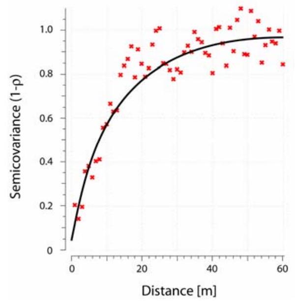
Fig. 29.3 Empirical semivariogram and fitted semivariance function for example soil data

Once an empirical semivariogram is produced, a predictive equation can be fitted to the data (see Fig. 29.3), and used as a model for spatial correlation in the applications described in this document.

29.4.3. Prior information on soil properties; Bayesian updating

Prior Information

In general, field parameters such as expected mean value, standard deviation and correlation parameters must be inferred from in situ tests. Usually prior information, especially regarding mean values, is available if classification into soil types is possible, based on collection of previous soil investigations on these soil types. In Table 29.3 and Table 29.4 a compilation is made of indicative prior estimates of soil properties for some selected soil categories, based on literature. Some national or regional geotechnical codes contain tables with prior indications on soil properties, which may differ from the indications in table Table 29.3 and Table 29.4, often due to differences of soil type classification and the regional geological characteristics.

Table 29.3 Prior indications of Soil properties of non cohesive soils

Non cohesive Soil type	Density	Dry Unit Weight \(\left[\mathrm{kN} / \mathrm{m}^{3}\right]\)	Saturated Unit Weight \(\left[\mathrm{kN} / \mathrm{m}^{3}\right]\)	Internal Friction \(\tan \left(\varphi^{\prime}\right)\)	Stiffness \(\left[\mathrm{MN} / \mathrm{m}^{2}\right]\)
Coarse gravel, Boulders	loose medium dense	15 - 17 17 - 18 18 - 20	19 - 20 20 - 21 21 - 23	0.65 - 0.73 0.70 - 0.83 0.78 - 0.90	150 - 300 150 - 300 250 - 350
Sand, gravel Uniform grain Size	loose medium dense	15 - 16 17- 18 18 - 19	19 - 20 20 - 21 21 - 22	0.58 - 0.65 0.65 - 0.73 0.70 - 0.83	30 - 100 50 - 150 100 - 200
Sand, gravel Non-uniform Grain size	loose medium dense	17 - 19 18 - 20 20 - 21	20 - 22 21 - 23 22 - 24	0.57 - 0.70 0.62 - 0.75 0.70 - 0.85	30 - 100 50 - 150 150 - 250
Sand Slightly Silty Silty		18 - 20 18 - 20	20 - 21.5 19.5 - 20.5	0.50 - 0.65 0.45 - 0.60	25 - 50 20 - 40

Table 29.4 Prior indications of soil properties of cohesive soils

Cohesive Soil type	Consistency	Saturated Unit Weight \(\left[\mathrm{kN} / \mathrm{m}^{3}\right]\)	Internal friction \(\tan (\varphi ’)\) (drained)	Cohesion (drained) \(\left[\mathrm{kN} / \mathrm{m}^{2}\right]\)	Undrained Shearing Strength \(\left[\mathrm{kN} / \mathrm{m}^{2}\right]\)	Stiffness (normally consolidated) \(\left[\mathrm{MN} / \mathrm{m}^{2}\right]\)
Inorganic cohesive soils, Plastic	soft stiff very stiff	16 - 18 17 - 19 20 - 22	0.27 - 0.36 0.27 - 0.36 0.27 - 0.36	0 - 5 5 - 15 15 - 30	10 - 20 20 - 50 50 - 100	1 - 2 2 - 4 4 - 10
Inorganic cohesive soils, Medium plastic	soft stiff very stiff	17 - 19 18 - 20 19 - 21	0.35 - 0.42 0.35 - 0.42 0.35 - 0.42	0 - 5 5 - 10 10 - 20	0 - 10 15 - 30 40 - 100	1 - 2 2 - 4 4 - 10
Inorganic cohesive soils, Weakly plastic		18 - 20	0.40 - 0.60	0 - 5	0 - 10	2 - 5
Boulder clay		20 - 24	0.52 - 0.64	20 - 30	-	200 - 700
Organic cohesive soils, Silt	soft stiff	13 - 18 14 - 19	0.24 - 0.28 0.24 - 0.28	0 - 5 5 - 10	5 - 20 15 - 30	0.2 - 0.5 0.5 - 1

Table 29.5 gives some indications of standard deviations of soil properties. These quantities refer to volumes affected by the testing device, with characteristic dimensions of some centimeters for laboratory test devices up to a few decimeters for field test devices. As these characteristic dimensions are small relative to characteristic dimensions of affected surfaces or volumes in geotechnical mechanisms, these standard deviations may be interpreted as standard deviations of soil property fluctuations “from point to point”.

Table 29.5 Indicative standard deviations of soil properties

Soil property	Standard deviation [% of expected mean value ]
Unit weight \(\left[\mathrm{kN} / \mathrm{m}^{3}\right]\)	5 - 10 %
Internal Friction \(\tan \left(\varphi^{\prime}\right)\) (drained)	10 - 20 %
Drained Cohesion \(\left[\mathrm{kN} / \mathrm{m}^{2}\right]\)	10 - 50 %
Undrained Shearing Strength \(\left[\mathrm{kN} / \mathrm{m}^{2}\right]\)	10 - 40 %
Stiffness \(\left[\mathrm{MN} / \mathrm{m}^{2}\right]\)	20 - 100 %

Distribution types

The assumption of normal (Gaussian) probability distributions for soil properties is most usual in geotechnical reliability analysis. Partly, this is supported by experimental evidence (e.g. [29.06], [29.07]) indicating that the normal distribution cannot be rejected for a wide variety of soil properties. Likely, however, this practice is also inspired by convenience of modeling. When performing probabilistic reliability analyses of soil structures the assumption of normality may lead to physical inconsistencies, e.g. negative design point values of shearing strengths. In order to avoid such inconsistencies it is recommended to assume log-normal distributions for soil properties which are strictly positive.

A log-normal field may be related to a normal field by appropriate transformation. The log normal field is represented by:

(29.41)\[p(\underline{x})=e^{u(\underline{x})}\]

where \(p(\underline{x})\) is the log-normal field, with expected mean value \(m_{p}\) and coefficient of variation \(V_{p}\), and where \(u(\underline{x})\) is a normal field with variance \(\sigma_{u}^{2}=\ln \left(1+V_{p}^{2}\right)\) and with expected mean value \(E[u]=\ln \left(m_{p}\right) -\frac{1}{2} \sigma_{u}{ }^{2}\). Then the equivalent normalized autocovariance function for the normal field is [Rackwitz, 2000]:

(29.42)\[\rho_{u}(\tau)=\frac{\ln \left(1+\rho_{p}(\tau) V_{p}^{2}\right)}{\ln \left(1+V_{p}^{2}\right)} \quad\left(\approx \rho_{p}(\tau) \quad \text { for } V_{p}^{2}<<1\right)\]

This implies the restriction \(\rho_{p}(\tau) V_{p}^{2}>-1\), in order to retain an admissible normalized autocovariance function \(\rho_{u}(\tau)\).

Consequently, log-normality of some (strictly positive) soil parameter \(p\) can be treated in a reliability analysis by replacing the field \(p(\underline{x})\) by \(\exp (u(\underline{x}))\), where statistics of the normal field \(u(\underline{x})\) are related to the statistics of \(p(\underline{x})\) according to the above given expressions.

Bayesian updating of prior information

Actual observations of a field property can be combined with prior information in order to update estimates of the field property statistics. Suppose prior information indicates a probability density distribution \(p d f^{\prime}\left(\underline{S_{p}}\right)\) for the statistics \(\underline{S_{p}}\) of the field property \(p\). Suppose further that a vector of observations \(\underline{P}\) is available. Then the Bayesian update reads (in generic form):

(29.43)\[p d f^{\prime \prime}\left(\underline{S}_{p} \mid \underline{P}\right)=C~p d f^{\prime}\left(\underline{S}_{p}\right) L\left(\underline{P} \mid p d f^{\prime}\left(\underline{S}_{p}\right)\right.\]

where \(p d f^{\prime \prime}\left(S_{p} \mid \underline{P}\right)\) is the posterior distribution of \(\underline{S}_{p}\) given the observations, \(L\left(\underline{P} \mid p d f^{\prime}\right.\left.\left(\underline{S}_{p}\right)\right)\) the likelihood function (the likelihood of the observations, given the prior pdf) and \(C\) a normalizing constant.

29.4.4. Uncertainties due to test imperfections

The results of laboratory or in situ tests are genrally affected by measurement related uncertainties, resulting from sample acquisition, specimen preparation and test imperfections. Thus the observed variability in test results originate from both intrinsic spatial varability of the soil, as well as from sampling disturbances and test imperfections. Assuming that no structural bias is introduced by sampling and testing procedures, one may proceed as follows.

Let \(\sigma_{r p}\) be the standard deviation related to sampling and test imperfections an \(\sigma_{p}\) the standard deviation related to intrinsic spatial variability. Assuming that sampling and testing imperfections are independent from intrinsic spatial variability, the total variance, as “read” from the tests equals:

(29.44)\[\sigma^{2}=\sigma_{r p}^{2}+\sigma_{p}^{2}\]

The standard deviation \(\sigma_{r p}\) is roughly to estimated in the order of 25 to 30 percents of the total standard deviation \(\sigma\) [29.08].

Sampling and test imperfections may be accounted for in the probabilistic field model by replacing the (intrinsic) field variance by the variance as “read” from the tests and replacing the theoretical normalized autocovariance function by:

(29.45)\[\begin{split}\begin{aligned} r_{p}(\Delta \underline{x}) & =1 & & \text { for } \Delta \underline{x}=\underline{0} \\ & =\alpha \rho_{f_{p}}(\Delta \underline{x}) & & \text { for } \Delta \underline{x} \neq \underline{0} \end{aligned}\end{split}\]

where \(\alpha\) is the estimated ratio of intrinsic field variance and the apparent field variance, as inferred from field observations, and \(r_{p}\) is the normalized autocovariance function for measured soil properties. According to the previously quoted magnitude of the standard deviation of sampling and test imperfections, \(\alpha\) will be in the order of 0.9 to 0.95. Consequently, sampling and test imperfections may be accounted for in the estimation of field statistics by using the normalized autocovariance function (29.45) for the evaluation of the covariance matrix \(\mathrm{R}\) in the statistical estimation procedure in sec. 29.4.1. and the Bayesian updating procedure in sec. 29.4.3..

Note that the function of (29.45) should be used only for modelling of measurements soil properties. If one is modelling the joint distribution of intrinsic soil properties, then the original \(\rho_{f_{p}}(\Delta \underline{x})\) function should be used. Note also that function (29.45) assumes the measurement errors to be independent; if this is not the case, then modifications to the equation will be neccessary.

29.5. Probabilistic Reliability Analysis of Geotechnical Structures

29.5.1. Uncertainties due to fluctuation of continuum properties

In order to apply soil models and soil model parameters, as defined in the previous sections, to geotechnical probabilistic analysis, the soil model must be fitted into the computation model for geotechnical analysis. Basically two categories of approaches can be distinguished, namely:

• full integration of the spatial fluctuation model for soil properties in the geotechnical computation model and

• reduction of the spatial fluctuation model for soil properties to dicrete parameters which fit directly into the (analytical) formulae of the geotechnical computation model.

Full integration:

This requires a revision of the underlying assumptions of the geotechnical computation model. For example, analytical formulas for bearing capacity are based on evaluation of limit state equilibrium along assumed rupture lines or surfaces. The spatial model for shear strength must be applied to these rupture figures. Equilibrium evaluation follows from integration or, more usual, discrete summation of the (stochastic) shear strengths along the rupture surface.
Stochastic Finite Element analysis belongs to this category.

Reduction of the Spatial Fluctuation Model:

This requires that the spatial fluctuation model is reduced to an expected mean value and a standard deviation which fits directly into the formulae framework of the geotechnical computation model. For example, the shear strength in a bearing capacity formula represents the average shear strengths along a rupture surface. Consequently the spatial model must be reduced to a single random variable, reflecting the average shear strength along this surface. In this case, variance reduction due to averaging, as described in sec. 29.3.4, must be taken into account. The variance of the single random variable reads:

(29.46)\[\sigma_{p}^{2}=\alpha \sigma^{2} \Gamma^{2}(S)+\sigma_{m_{p}}^{2}\]

where \(\alpha\) is the (estimated) ratio of the intrinsic field fluctuation variance and the apparent field fluctuation variance (see eq. (29.45)), \(\sigma^{2}\) the apparent field fluctuation variance, \(\Gamma^{2}\) the variance reduction factor (see section 29.3.3.) and \(\sigma_{m p}^{2}\) is the variance of statistical uncertainty of the mean value (see section 29.4.1.).

29.5.2. Computation model uncertainties

Computation models, especially in the geotechnical field, may itself contain considerable uncertainties. Uncertainties may be due to various reasons, e.g.(over)simplification of the equilibrium or deformation analysis and neglecting to account for 3-D effects.

A simple way of taking computation model uncertainties into account is by multiplication of the computed responses of the soil or the foundation with additional random variables. Expected mean values and standard deviations of these factors may be assessed on the basis of empirical or experimental data, on comparison with more advanced computation models or, in case of lack of specific and explicit data, on engineering judgement (expert opinion).

Table 29.6 gives some rough figures for expected means and standard deviations for some frequently used geotechnical computation models. These factors relate to the resistance component in the computation model. Generally computation model uncertainty may depend on the situation at hand, e.g. homogeneous or heterogeneous soil profiles, type of tests for the assessment of soil property data, etc.

Table 29.6 Indicative computation model uncertainty factors

Type of problem	Type of calculation model	Expected mean	Standard deviation
Embankment slope stability Homogeneous soils Non homogeneous soils	Failure arc analysis (e.g. Bishop, Spencer, etc.), 2-D FEM	1.1 1.1	0.05 0.10
Stability of retaining (sheetpiled) walls	Brinch Hansen, Blum, Elastic/plastic spring supported beam model	1.0	0.10
Shallow Foundations Stability: Homogeneous soil profile Non homogeneous soil profile Settlement:prediction	Brinch Hansen	1.0 1.0 1.0	0.15 0.20 0.20 - 0.30
Foundation piles (driven) Point bearing capacity Shaft resistance	CPT based empirical design rules	1.0 1.0	0.25 0.15
Embankment settlement prediction		1.0	0.20

Instead of one uncertainty factor for the computational model as a whole, one may consider the use of partial uncertainty factors related to components of the computation model. For example uncertainty factors related to active and passive earth pressure and related to stress distribution in the analysis of stability of retaining walls. Such approach allows for differentiation of uncertainty factors and better transparency of the effects of uncertain aspects in the analysis.

29.5.3. Uncertainties of soil stratigraphy

A soil stratigraphy must be defined on the basis of data from geotechnical survey. This consists of:

• assessment of the main pattern of (statistically) homogeneous layers

• assessment of locally present smaller soil units

• assessment of other local phenomena, such as discontinuities

• classification of each soil unit

As geotechnical data reflects spatial point or line information, boundaries of soil units in between survey point or lines must be estimated by interpolation. Uncertainties regarding the position of layer boundaries at interpolated locations may be of importance in a geotechnical analysis. Sometimes a geostatistical approach may be helpfull to estimate inaccuracies of layer boundary positions. However, in many occasions the available soil data is insufficient to infer the spatial covariance structure of fluctuations of layer boundaries, needed for such approach.

A different kind of uncertainty results from the fact that small size soil units or other local phenomena, though not revealed by the soil data, may nonetheless be present. Based on knowledge of the regional geology (and the way local phenomena may affect functional performance of the structure to be designed) it must be decided whether or not such a local phenomenon may be disregarded. If not, it must be assumed to be present and it must be taken into account in the design of the structure. The detection of this type of feature using a finite number of soil samples is addressed in the field of search theory [29.09], [29.010].

Both types of uncertainty can be accounted for in a probabilistic geotechnical analysis, assuming a sequence of potential scenario’s of the soil stratigraphy. Based on soft information, i.e. geological background information, and hard soil data of the site different scenario’s of the soil stratigraphy can be developed, each one of which fully matches the available hard soil data, however with generally different degrees of belief. Assessment of degrees of belief, i.e. estimated probabilities that a particular soil stratigraphical scenario is correct, is up to (subjective) estimation by the geologist.

Starting from each of the stratigraphical scenario’s, a conditional probabilistic reliability analysis of some soil property related event, \(F\), e.g. failure, may be performed, using stochastic soil parameter models as discussed previously. The total prior probability of failure equals:

(29.47)\[P[F]=\sum_{i=1}^{N} P\left[F \mid S_{i}\right]~P\left[S_{i}\right]\]

where \(P\left[F \mid S_{i}\right]\) denotes the conditional probability of failure, assuming that the stratigraphic scenario \(S_{i}\) is correct, and \(P\left[S_{i}\right]\) the estimated probability that the scenario is correct. \(`\mathrm{N}\) is the number of scenario’s of the soil stratigraphy.

In cases with unlikely but very unfavorable scenario’s of the stratigraphy, significant overdimensioning of the design of the structure may be the result. The alternative option is to conduct additional soil investigation, which either reveals that an unfavorable scenario is a true scenario, or yields better confidence that it is not present. In the latter case this results in reduction of the probabilities, \(P\left[S_{i}\right]\), of unfavorable scenario’s.

References

[29.01] (1,2)

E.H. Vanmarcke. Probabilistic modeling of soil profiles. ASCE Journal of the Geotechnical Engineering Division, 1977. Also: E.H. Vanmarcke, Random Fields – Analysis and Synthesis, MIT Press, Cambridge, 1983.

[29.02]

R. Rackwitz. Reviewing probabilistic soils modelling. Computers and Geotechnics, 26(3-4):199–223, 2000.

[29.03] (1,2)

T. Vrouwenvelder and E. Calle. Measuring spatial correlation of soil properties. Heron, 48(nr 4):297–311, 2003. www.heron.tudelft.nl.

[29.04]

P. Goovaerts. Geostatistics for natural resources evaluation. Oxford University Press, New York, 1997.

[29.05]

The Stanford Geostatistical Modeling Software (S-GeMS). S-GeMS. http://sgems.sourceforge.net/, 2006.

[29.06]

P. Lumb. The variability of natural soils. Canadian Geotechnical Journal, III(2):74–94, 1966.

[29.07]

E. Schultze. Frequency distribution and correlation of soil properties. In Proceedings of the 1st International Conference on Applications of Statistics And Probability to Soil and Structural Engineering, 371–387. Hong Kong, 1971.

[29.08]

C. Cherubini. Data and considerations on the variability of geotechnical properties of soils. In C. Guedes Soares, editor, Advances in Safety and Reliability, Proceedings of the ESREL '97, volume 2, 1583–1591. Lisbon, 1997.

[29.09]

G.B. Baecher and J.T. Christian. Reliability and statistics in geotechnical engineering. J. Wiley, Chichester, West Sussex, England; Hoboken, NJ, 2003.

[29.010]

S.J. Benkoski, M.G. Monticino, and J.R. Weisinger. A survey of the search theory literature. Naval Research Logistics, 38:469–494, 1991.

[29.011]

W.H. Tang. Probabilistic evaluation of penetration resistances. ASCE Journal of the Geotechnical Engineering Division, 105(GT 10):1173–1191, 1979.

[29.012]

A. Asoaka and D.A. Grivas. Spatial variability of the undrained strength of clays. ASCE Journal of the Geotechnical Engineering Division, 108(GT5):743–756, 1982.

[29.013]

D.J. Mulla. Estimating spatial patterns in water content, matric suction and hydraulic conductivity. Soil Science Society of America Journal, 52:1547–1553, 1988.

[29.014]

M. Ronold. Random field modeling of foundation failure modes. Journal of Geotechnical Engineering, April 1990.

[29.015]

K. Unlu, D.R. Nielsen, J.W. Biggar, and F. Morkoc. Statistical parameters characterizing variability of selected soil hydraulic properties. Soil Science Society of America Journal, 54:1537–1547, 1990.

[29.016]

M. Soulié, P. Montes, and V. Silvestri. Modeling spatial variability of soil parameters. Canadian Geotechnical Journal, 27:617–630, 1990.

[29.017]

K.R. Rehfeldt, J.M. Boggs, and L.W. Gelhar. Field study of dispersion in a heterogeneous aquifer, 3-d geostatistical analysis of hydraulic conductivity. Water Resources Research, 28(12):3309–3324, 1992.

[29.018]

M.S. Rosenbaum. The use of stochastic models in the assessment of a geological database. Quarterly Journal of Engineering Geology, 20:31–40, 1987.

[29.019]

K.M. Hess, S.H. Wolf, and M.A. Celia. Large scale natural gradient tracer test in sand and gravel, cape cod, massachusetts 3. hydraulic conductivity variability and calculated macrodispersivities. Water Resources Research, 28(8):2011–2017, 1992.

[29.020]

P. Chiasson, J. Lafleur, M. Soulié, and K.T. Haw. Characterizing spatial variability of clay by geostatistics. Canadian Geotechnical Journal, 32:1–10, 1995.

Appendix 35.7.A: Scales of Fluctuation

Source	Soil Property	Purpose	Applied Spatial model type	Correlation radius
[29.011]	Marine clay, average cone resistance (CPT) from 0 - 3m below sea bottom. Different levels	Design skirts offshore platform	Gaussian	\(\delta_\mathrm{h}=\) 55 m \(\delta_\mathrm{h}=\) 35 - 60 m
[29.012]	Undrained shear strength	Modeling vertical spatial variability	Exponential	\(\delta_\mathrm{v}=\) 2.5 - 6 m
[29.013]	Surface temperature Water content Penetrometer resistance Sand content (sandy clay) Clay content	Prediction of water content	Variogram, spherical	\(\delta_\mathrm{h}=\) 50 - 70 m \(\qquad\) 40 - 60 m \(\qquad\) 40 - 70 m \(\qquad\) 60 - 80 m \(\qquad\) 40 - 60 m
[29.014]	Shearing strength (clay)	Capacity of tension piles	Gaussian	\(\delta_\mathrm{v}=\) 2 m
[29.015]	ln(K\(_{\text{unsaturated}}\)) Soil parameter (unspec) Water capacity	Comparison of methods for assesment of scale of correlation		\(\delta_\mathrm{h,\ln K}=\) 12 – 16 m \(\delta_\mathrm{h,par}=\) 40 m \(\delta_\mathrm{h,cap}=\) 12 – 16 m
[29.016]	Shear strength	Modeling spatial variability for dam design	Exponential	\(\delta_\mathrm{v}=\) 2 m, \(\delta_\mathrm{h}=\) 20 m
[29.017]	ln Permeability	Modeling spatial variability, tracer tests	Exponential	Flowmeter: \(\delta_\mathrm{v}=\) 3.2 m, \(\delta_\mathrm{h}=\) 25 m Several tests: \(\delta_\mathrm{v}=\) 1.5 - 3 m, \(\delta_\mathrm{h}=\) 25 – 50 m
Honjo et al 1991	Unconf. compr. strength	Slope stability evaluation	Exponential	\(\delta_\mathrm{v}=\) 4 m, \(\delta_\mathrm{h}=\) 80 m
[29.018]	Thickness of natural deposit		Variogram, spherical	\(\delta_\mathrm{h}=\) 750 m
[29.019]	ln Permeability	Contaminant migration	Exponential	\(\delta_\mathrm{v}=\) = 0.2 – 1.0 m, \(\delta_\mathrm{h}=\) 2 – 10 m
[29.020]	CPT, vane shear strength	Modeling spatial variability	Variogram, spherical	\(\delta_\mathrm{v}=\) 1.5 m
[29.03]	CPT, cone resistance deep glacial sands	Modeling spatial variability	Gaussian	\(\delta_\mathrm{h}=\) 20 – 35 m