28. Properties of Timber

List of most important symbols:

\(\begin{array}{ll}R_{m} \quad & \text { bending strength } \\ E_{m} \quad & \text { bending MOE } \\ \rho_{\text {den }} \quad & \text { density } \\ R_{t, 0 / 90} \quad & \text { tension strength } \\ E_{t, 0 / 90} \quad & \text { tension MOE } \\ R_{c, 0 / 90} \quad & \text { compression strength } \\ E_{c, 0 / 90} & \text { compression MOE } \\ R_{v} \quad & \text { shear strength } \\ G_{v} \quad & \text { shear modulus } \\ R_{h, 0 / 90} \quad & \text { embedding strength } \\ \sigma \quad & \text { stress } \\ \varepsilon \quad & \text { strain } \\ E_{t} & \text { tension MOE } \\ E_{c} & \text { compression MOE } \\ R_{c} \quad & \text { compression strength } \\ R_{c, y} \quad & \text { asymptotic final compression strength } \\ R_{t} \quad & \text { tension strength } \\ \varepsilon_{u} \quad & \text { ultimate strain } \\ S(t) \quad & \text { load history } \\ \omega & \text { humidity } \\ \tau \quad & \text { temperature } \\ T \quad & \text { time } \\ \alpha \quad & \text { strength modification function } \\ \alpha_{D}, \alpha_{\kappa} \quad & \text { damage state } \\ \delta \quad & \text { stiffness modification function } \\ R_{0} \quad & \text { failure stress under short term ramp loading } \\ X_{M} \quad & \text { model uncertainty } \\ \hat{x} \quad & \text { tests data } \\ i \quad & \text { strength indicator }\end{array}\)

28.1. Introduction

Timber is a rather complex building material. Its properties are highly variable, spatially and in time. In structural engineering, material properties of timber are the stress and stiffness related properties of standard test specimen under given (standard) loading and climate conditions and the timber density. Timber is a graded material. Due to the grading process, the material properties are associated with some control scheme, whereas only the so-called reference material properties are considered explicitly. The so-called other material properties are only assessed implicitly. The distinction between reference properties and other properties is made as illustrated in Fig. 28.1 . The bending strength \(R_{m}\), the bending modulus of elasticity \(E_{m}\) and the timber density \(\rho_{d e n}\) are referred to as the reference material properties.

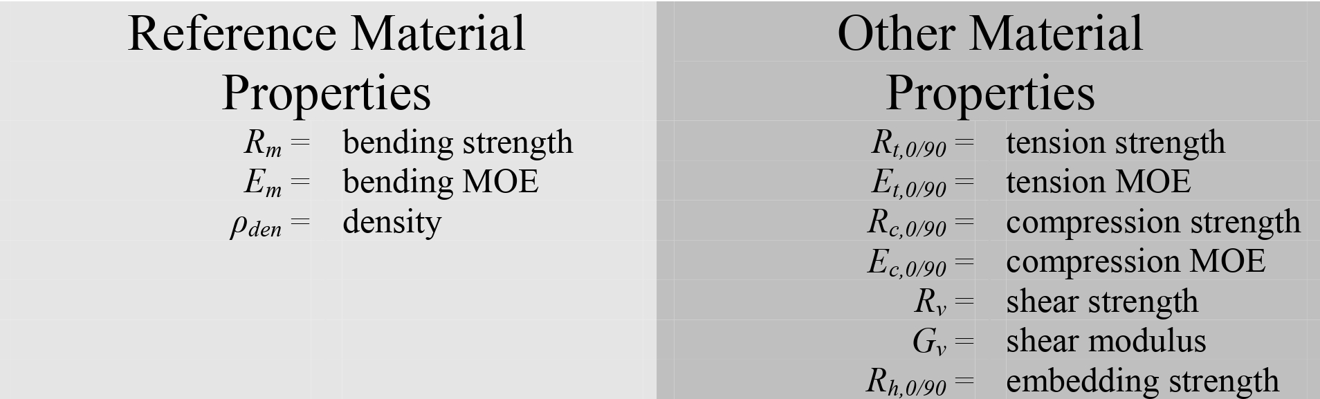
Fig. 28.1 Reference material properties and other material properties.

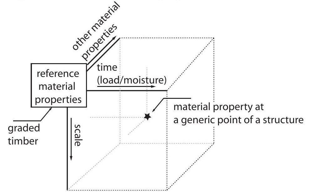
Fig. 28.2 Outline of the modelling of timber material properties.

When modelling timber material properties in a structure, i.e. at any generic point, in time and in space, several issues have to be taken into account. As illustrated in Fig. 28.2 the cornerstone of the modelling of timber material properties are the reference material properties under test conditions. The material property of interest at any generic point may deviate in terms of type (‘other material properties’), of dimensions (‘scale’) and of specific loading and climate conditions (‘time (load/moisture)’).

The models in this model code relate to solid structural timber and are predominantly based on test programs and investigations considering European and North American softwoods. For some other softwoods and especially for hardwood the underlying assumptions are less appropriate.

28.2. Basic Model

28.2.1. Stress-strain relationship

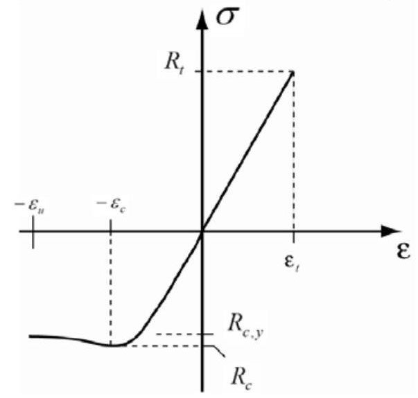
Fig. 28.3 Stress-strain relation according to Glos [28.01]. A simplified linear elastic-plastic stressstrain curve is shown with thin line.

In Fig. 28.3 an idealised stress-strain relationship under axial load is shown for \(\underline{\text{small clear timber specimens}}\), according to Glos, [28.01]. In tension there is a linear relationship described by the modulus of elasticity \(E_{t}\). In compression the relation is described by the initial modulus of elasticity \(E_{c}\), the compression strength \(R_{c}\), the asymptotic final compression strength \(R_{c, y}\), the strain \(\varepsilon_{c}\) at maximum stress and the ultimate strain \(\varepsilon_{u}\). The following empirical relation is assumed:

(28.1)\[\begin{split}\sigma(\varepsilon)=\left\lbrace \begin{array}{ccc}\frac{\varepsilon+k_{1} \varepsilon^{N}}{k_{2}+k_{3} \varepsilon+k_{4} \varepsilon^{N}} & \text { for } & -\varepsilon_{u} \leq \varepsilon \leq 0 \\ \\ E_{t} \varepsilon & \text { for } & 0 \leq \varepsilon \leq \varepsilon_{t}\end{array}\right.\end{split}\]

where

(28.2)\[k_{1}=\frac{R_{c, y}}{(N-1) \cdot E_{c} \cdot \varepsilon_{c}^{(N-1)}\left(1-R_{c, y} / R_{c}\right)}\]

(28.3)\[k_{2}=\frac{1}{E_{c}}\]

(28.4)\[k_{3}=\frac{1}{R_{c}}-\frac{N}{(N-1) \cdot E_{c} \cdot \varepsilon_{c}}\]

(28.5)\[k_{4}=\frac{k_{1}}{R_{c, y}}\]

Conditions for (28.1):

(28.6)\[R_{c, y} \leq R_{c}-1[\mathrm~{\text{MPa}}] \qquad \varepsilon_{c} \geq \frac{N}{(N-1)} \frac{R_{c}}{E_{c}}\]

Typical values for the parameters are:
\(R_{c, y} / R_{c} \approx 0.8 \qquad \varepsilon_{c}=0.8-1.2 \% \qquad \varepsilon_{u} \approx 3 \varepsilon_{c \qquad }N=7\)

For \(\underline{\text{structural timber}}\), the force-deformation relationship can be different.

28.2.2. Basic Material Properties

The reference properties of structural timber determined from standard tests are:

• the bending strength \(R_{m, t}\) in [MPa] and the

• bending modulus of elasticity \(E_{m, t}\) in [MPa],
  both measured on short-term standard test specimens evaluated according to ISO 8375 [28.02] with symmetrical 4-point bending test, span \(18 h(3 \cdot 6 \cdot h)\) with \(h \approx 150 \mathrm{~mm}\), ramp load test duration \(300 \pm 120 \mathrm{~s}\), specimen conditioned at nominal climate, \(20 \pm 2^{\circ} \mathrm{C}, 65 \pm 5 \%\) relative humidity.

• timber density \(\rho_{d e n, t}\) in \(\left[\mathrm{kg} / \mathrm{m}^{3}\right]\), measured according to ISO 3131 [28.03] from a disc of full cross section, free of knots and resin pockets.

The reference material properties are sensitive to the deviations from the standard test conditions. The reference material properties of a cross section in situ (i.e. at any generic point in time and in space) are estimated as:

Bending moment capacity in situ, \(R_{m}\) :

(28.7)\[R_{m}=\alpha(E x(S, \omega, \tau, T)) R_{m, 0}\]

Bending MOE in bending in situ, \(E_{m}\) :

(28.8)\[E_{m}=E_{m, 0} /(1+\delta(E x(S, \omega, \tau, T)))\]

Density in situ, \(\rho_{\text {den }}\) :

(28.9)\[\rho_{d e n}=\rho_{\text {den }, 0}\]

where

\(\operatorname{Ex}(S, \omega, \tau, T)\) is the exposure of the structure to loads \(S\), humidity \(\omega\) and temperature \(\tau\), in the time interval \([0, T]\)

\(\alpha(E x(.))\) is a strength modification function, in general defined for a particular set of exposures

\(\delta(E x(.))\) is a stiffness modification function, in general defined for a particular set of exposures.

\(R_{m, 0}, E_{m, 0}\) and \(\rho_{\text {den, } 0}\) are the bending moment capacity, the modulus of elasticity and the density of a cross section under test conditions. It is assumed that these properties are equal to the properties of the corresponding standard test specimen; i.e. it is assumed that within test specimen and within structural components these properties are constant.

Other material properties are estimated based on the reference material properties, see next section.

28.3. Probabilistic model

28.3.1. Expected values and COV

Expressions for the expected values \(E[.]\) and the coefficient of variation \(\operatorname{COV}[.]\) are given in Table 28.1 for Nordic softwood.

Table 28.1 Relation reference properties - other properties

Property	Expected Values \(E[X]\)	Coefficient of variation \(\operatorname{COV}[X]\)
Tension strength par. to the grain, \(R_{t, 0}:\)	\(E\left[R_{t, 0}\right]=0.6 E\left[R_{m}\right]\)	\(\operatorname{COV}\left[R_{t, 0}\right]=1.2 \operatorname{COV}\left[R_{m}\right]\)
Tension strength perpendicular to the grain, \(R_{t, 90}:\)	\(E\left[R_{t, 90}\right]=0.015 E\left[\rho_{\text {den }}\right]\)	\(\operatorname{COV}\left[R_{t, 90}\right]=2.5 \operatorname{COV}\left[\rho_{\text {den }}\right]\)
MOE - tension par. to the grain, \(E_{t, 0}\) :	\( E\left[ E_{t, 0}\right]=E\left[E_{m}\right]\)	\(\operatorname{COV}\left[ E_{t, 0}\right]=\operatorname{COV}\left[E_{m}\right]\)
MOE - tension perpendicular to the grain, \(E_{t, 90}\) :	\(E\left[E_{t, 90}\right]=E\left[E_{m}\right] / 30\)	\(\operatorname{COV}\left[E_{t, 90}\right]=\operatorname{COV}\left[E_{m}\right]\)
Compression strength parallel to the grain, \(R_{c, 0}\) :	\(E\left[R_{c, 0}\right]=5 E\left[R_{m}\right]^{0.45}\)	\(\operatorname{COV}\left[R_{c, 0}\right]=0.8 \operatorname{COV}\left[R_{m}\right]\)
Compression strength perpendicular to the grain, \(R_{c, 90}:\)	\(E\left[R_{c, 90}\right]=0.008 E\left[\rho_{d e n}\right]\)	\(\operatorname{COV}\left[R_{c, 90}\right]=\operatorname{COV}\left[\rho_{\text {den }}\right]\)
Shear modulus, \(G_{v}:\)	\(E\left[G_{v}\right]=E\left[E_{m}\right] / 16\)	\(\operatorname{COV}\left[G_{v}\right]=\operatorname{COV}\left[E_{m}\right]\)
Shear strength, \(R_{v}:\)	\(E\left[R_{v}\right]=0.2 E\left[R_{m}\right]^{0.8}\)	\(\operatorname{COV}\left[R_{v}\right]=\operatorname{COV}\left[R_{m}\right]\)

The relations are derived for standard test specimen properties tested under reference conditions. However, it is assumed that the relations can be used at any level, i.e. for components of any size and/or for other climate and load conditions.

28.3.2. Distribution types

The distribution type and the recommended coefficient of variation ( \(\text{COV}\) ) of the basic material properties for European softwood are given in Table 28.2 as prior values corresponding to a number of tests equal to 10 .

Table 28.2 Probabilistic models for reference properties for structural timber

	Distribution	\(\text{COV}\)
Bending strength \(R_{m}\)	Lognormal	0.25
Bending MOE: \(E_{m}\)	Lognormal	0.13
Density \(\rho_{\text {den }}\)	Normal	0.1

The distribution types for the other basic material properties are given in Table 28.3.

Table 28.3 Distribution functions for other material properties for structural timber

Property	Distribution Function
Tension strength par. to the grain, \(R_{t, 0}:\)	Lognormal
Tension strength perpendicular to the grain, \(R_{t, 90}:\)	2-p Weibull
MOE - tension par. to the grain, \(E_{t, 0}:\)	Lognormal
MOE - tension perpendicular to the grain, \(E_{t, 90}:\)	Lognormal
Compression strength parallel to the grain, \(R_{c, 0}:\)	Lognormal
Compression strength perpendicular to the grain, \(R_{c, 90}:\)	Normal
Shear modulus, \(G_{v}:\)	Lognormal
Shear strength, \(R_{v}:\)	Lognormal

28.3.3. Correlation coefficients

Table 28.4 Correlation coefficient matrix

	\(E_{m}\)	\(\rho_{\text {den }}\)	\(R_{t, 0}\)	\(R_{t, 90}\)	\(E_{t, 0}\)	\(E_{t, 90}\)	\(R_{c, 0}\)	\(R_{c, 90}\)	\(G_{v}\)	\(R_{v}\)
\(R_{m}\)	0.8	0.6	0.8	0.4	0.6	0.6	0.8	0.6	0.4	0.4
\(E_{m}\)		0.6	0.6	0.4	0.8	0.4	0.6	0.4	0.6	0.4
\(\rho_{d e n}\)			0.4	0.4	0.6	0.6	0.8	0.8	0.6	0.6
\(R_{t, 0}\)				0.2	0.8	0.2	0.5	0.4	0.4	0.6
\(R_{t, 90}\)					0.4	0.4	0.2	0.4	0.4	0.6
\(E_{t, 0}\)						0.4	0.4	0.4	0.6	0.4
\(E_{t, 90}\)							0.6	0.2	0.6	0.6
\(R_{c, 0}\)								0.6	0.4	0.4
\(R_{c, 90}\)									0.4	0.4
\(G_{v}\)										0.6

The relations to other material properties are given in Table 28.1. Indicative values of the correlation coefficient matrix are given in Table 28.4 . The values in Table 28.4 are quantified by judgment (COST E24 [28.04]), such that \(0.8 \leftrightarrow\) high correlation, \(0.6 \leftrightarrow\) medium correlation, \(0.4 \leftrightarrow\) low correlation, \(0.2 \leftrightarrow\) very low correlation.

28.3.4. Failure types

Failure modes related to the different strength parameters are characterized as brittle, ductile or ductile with reserve strength, see Table 28.5.

Table 28.5 Failure types for different failure modes for structural timber

Property	Failure type
Bending, \(R_{m}:\)	Ductile \({ }^{1)}\)
Tension parallel to the grain, \(R_{t, 0}:\)	Brittle
Tension perpendicular to the grain, \(R_{t, 90}:\)	Brittle
Compression parallel to the grain, \(R_{c, 0}:\)	Ductile
Compression perpendicular to the grain, \(R_{c, 90}:\)	Ductile with reserve
Shear, \(R_{v}:\)	Brittle

\(1)\) for lower grade timber the failure mode can be brittle.

28.3.5. Strength and Stiffness Modification Functions

Values for the strength modification function \(\alpha(.)\) are quantified for discrete exposures \(\operatorname{Ex}(S, \omega, \tau, T)\) as specified in Table 28.6. The particular sets of exposures are defined as in EC 5 [28.05]; different load duration classes and different service classes (sc) depending on the expected moisture content (mc) of the timber (sc 1, 2, 3 is associated with mc \(<12 \%,<20 \%\) and \(>20 \%\)). The values for \(\alpha(.)\) are taken from EC 5.

Table 28.6 Strength modification function table for constant loads with different duration

sc	Permanent \((T>10~\text{years} )\)	Long term \((10>T>0.5~\text{years})\)	Medium term \((6>T>0.25~\text{month})\)	Short term \((T<~\text{1 week})\)	Instantaneous
\(1 / 2\)	\(\alpha=0.6\)	\(\alpha=0.70\)	\(\alpha=0.80\)	\(\alpha=0.9\)	\(\alpha=1.1\)
\(3\)	\(\alpha=0.5\)	\(\alpha=0.55\)	\(\alpha=0.65\)	\(\alpha=0.7\)	\(\alpha=0.9\)

Values for the stiffness modification function \(\delta(.)\) are quantified for discrete exposures \(\operatorname{Ex}(S, \omega, \tau, T)\) as specified in Table 28.7. The particular sets of exposures are defined as in EC 5 [28.05]. The values for \(\delta(.)\) are taken from EC 5.

Table 28.7 Stiffness modification function table for constant loads with different duration

sc	Permanent \((T>10~\text{years} )\)	Long term \((10>T>0.5~\text{years})\)	Medium term \((6>T>0.25~\text{month})\)	Short term \((T<~\text{1 week})\)	Instantaneous
1	\(\delta=0.6\)	\(\delta=0.5\)	\(\delta=0.25\)	\(\delta=0.0\)	\(\delta=0.0\)
2	\(\delta=0.8\)	\(\delta=0.5\)	\(\delta=0.25\)	\(\delta=0.0\)	\(\delta=0.0\)
3	\(\delta=2.0\)	\(\delta=1.5\)	\(\delta=0.75\)	\(\delta=0.3\)	\(\delta=0.0\)

28.3.6. Glued laminated timber

The stochastic model for glued laminated timber is related to the strength parameters for whole structural elements, and not to the strength parameters for the single laminates and the glue. In Table 28.8 a prior probabilistic model for the material strength properties is given corresponding to a number of tests equal to 10. In Table 28.9 failure types for different failure modes are shown.

Table 28.8 Probabilistic models for properties for glued laminated timber

	Distribution	\(COV\)
Bending strength: \(R_{m}\)	Lognormal	0.15
Bending MOE: \(E_{m}\)	Lognormal	0.13
Tension strength par. to the grain: \(R_{t, 0}\)	Lognormal
Tension strength perpendicular to the grain: \(R_{t, 90}\)	2-p Weibull
MOE - tension par. to the grain: \(E_{t, 0}\)	Lognormal
MOE - tension perpendicular to the grain: \(E_{t, 90}\)	Lognormal
Compression strength parallel to the grain: \(R_{c, 0}\)	Lognormal
Compression strength perpendicular to the grain: \(R_{c, 90}\)	Normal
Shear modulus: \(G_{v}\)	Lognormal
Shear strength: \(R_{v}\)	Lognormal
Density: \(\rho_{d e n}\)	Normal	0.1

Table 28.9 Failure types for different failure modes for glued laminated timber

Property	Failure type
Bending: \(R_{m}\)	Brittle
Tension parallel to the grain: \(R_{t, 0}\)	Brittle
Tension perpendicular to the grain: \(R_{t, 90}\)	Brittle
Compression parallel to the grain: \(R_{c, 0}\)	Ductile
Compression perpendicular to the grain: \(R_{c, 90}\)	Ductile with reserve
Shear: \(R_{v}\)	Brittle

28.3.7. Model Uncertainties for Different Ultimate Limit States

The model uncertainties cover deviations and simplifications related to the probabilistic modelling and the limit state equations. The reference properties are determined by standardized tests. Therefore, model uncertainties related to estimation of other material parameters (e.g. tension and compression strengths) have to be accounted for. Geometrical deviations from specified dimensions, durations of load and moisture effects (damage accumulation) also contribute to model uncertainties if not explicitly accounted for in the probabilistic modelling. Furthermore, the idealized and simplified limit state equations introduce model uncertainties. In Table 28.10 values for model uncertainties are shown. The model uncertainty depends on the limit state (bending or e.g. combined stress effects) and how much the actual condition deviates from the standard test conditions.

Table 28.10 Model uncertainties for component load bearing capacity

	Mean	Standard deviation	Distribution
Without load duration effects	1	0.05 - 0.10	Lognormal
With load duration effects, eq. (28.16)-(28.17)	1	0.10	Lognormal

28.4. Refinements of the probabilistic model

28.4.1. Modeling the Spatial Variation of Timber Properties

Bending moment capacity

Following a model proposed by Isaksson [28.06], the bending strength \(R_{m, i j}\) at a particular point \(j\) in the component \(i\) of a structure/batch is given as:

(28.10)\[R_{m, i j}=\exp \left(v+\varpi_{i}+\chi_{i j}\right)\]

where

\(v\) is the unknown logarithm of the mean strength of all sections in all components, see Fig. 28.4

\(\varpi_{i}\) is the difference between the logarithm of the mean strength of the sections within a component \(i\) and \(v ; \varpi_{i}\) is normal distributed with mean value equal to zero and standard deviation \(\sigma_{\sigma}\)

\(\chi_{i j}\) is the difference between the strength weak section \(j\) in the beam \(i\) and the value \(v+\varpi_{i} ; \chi_{i j}\) is normal distributed with mean value equal to zero and standard deviation \(\sigma_{\chi}\). \(\varpi_{i}\) and \(\chi_{i j}\) are statistically independent.

The bending strength \(R_{m, i j}\) is the bending strength of a particular cross section. \(R_{m, i j}\) is lognormal distributed.

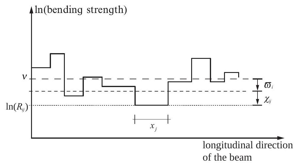
Fig. 28.4 Section model for the longitudinal variation of bending strength

It is assumed that the bending strength of a cross section is related with the bending strength of a test specimen \(R_{m, t}\) as:

(28.11)\[R_{m, 0}=R_{m, t}^{\vartheta}\]

where \(\vartheta\) is a constant depending on the applied bending test standard and the type of timber.

The bending moment capacity \(R_{m, 0}\) is assumed to be constant within one section. The discrete section transition is assumed to be Poisson distributed, thus the section length \(X\) follows an exponential distribution with mean value \(1 / \lambda\). A realization of \(X, x_{j}\) is illustrated in Fig. 28.4.

For Nordic spruce the following information basis can be given (Isaksson [28.06]): The variation of the logarithm of the bending capacity \(\ln \left(R_{m, 0}\right)\) is related by \(40 \%\) to the variable \(\varpi\) and by \(60 \%\) to the variable \(\chi\). The expected length of a section is \(1 / \lambda=480 \text{~mm}\).

Table 28.11 ϑ -values for the estimation of the strength of weak sections (for Nordic Spruce)

	EN	US	AUS
\(\vartheta=\)	1.05	1.03	1.02

Note: \(\vartheta\)-values should be used in connection with strength values in [MPa].

The different values for \(\vartheta\) given in Table 28.11 are due to the different definitions of bending strength of test specimen. The values are derived by simulations, see Köhler [28.07].

For the bending modulus of elasticity and the density no within component variation is assumed.

28.4.2. Duration of Load Effect

The mechanism leading to strength reduction of a timber member under sustained load is referred to as creep rupture and is modelled by so-called cumulative damage models with the general form:

(28.12)\[\frac{d \alpha_{D}}{d t}=h\left(S(t), R_{0}, \alpha_{D}, \boldsymbol{\theta}\right) \quad \text { for } \quad 0 \leq \alpha_{D} \leq 1\]

where \(t\) is time, \(\alpha_{D}\) is the damage state variable which commonly ranges from 0 (no damage) to 1 (failure), the function \(h(.)\) contains parameters \(\boldsymbol{\theta}\) that must be determined from experiment observations, \(S(t)\) is the applied stress and \(R_{0}\) the failure stress under short term ramp loading.

Three different models are proposed:

1. The model referred to as the Gerhards model [28.08]:

(28.13)\[\frac{d \alpha_{D}}{d t}=\exp \left(-a_{D}+b_{D} \frac{S(t)}{R_{0}}\right) \quad \text{for} \quad 0 \leq \alpha_{D} \leq 1\]

2. The model referred to as the Foschi and Yao model [28.09]:

(28.14)\[\begin{split}\begin{aligned} \frac{d \alpha_{D}}{d t} & =a_{D}\left(\frac{S(t)}{R_{0}}-\eta_{D}\right)^{b_{D}}+c_{D}\left(\frac{S(t)}{R_{0}}-\eta_{D}\right)^{d_{D}} \alpha_{D}(\mathrm{t}) & & \text { for } \frac{S(t)}{R_{0}} \geq \eta_{D} \\ \\ \frac{d \alpha_{D}}{d t} & =0 & & \text { for } \frac{S(t)}{R_{0}}<\eta_{D} \end{aligned}\end{split}\]

3. The model referred to as the Nielsen model [28.010]:

(28.15)\[\frac{d \alpha_{\kappa}}{d t}=\alpha_{\kappa}\left(\frac{S(t)}{R_{0}}\right)^{2}\left(\left(\alpha_{\kappa}\left(\frac{S(t)}{R_{0}}\right)^{2}\right)^{-1}-1\right)^{-\frac{1}{\mathrm{~b}_{\mathrm{D}}}} \text { for } 0 \leq \alpha_{\kappa} \leq\left(\frac{S(t)}{R_{0}}\right)^{-2}\]

where \(\alpha_{D}, \alpha_{\kappa}\) are the damage state variables, \(a_{D}, b_{D}, c_{D}, d_{D}, \eta_{D}\) are model parameters fitted to experimental results e.g. as in Sørensen et al. [28.011] and Köhler and Svensson [28.012].

For model 1) and 2) a time invariant limit state function can be formulated:

(28.16)\[g(T)=1-X_{M} \alpha_{D}(S(T))\]

where \(X_{M}\) is the model uncertainty, see Table 28.10. \(\alpha_{D}(S(T))\) at time \(T\) is obtained using the damage accumulation models 1 ) or 2) with the load time history \(S(t), 0 \leq t \leq T\).

For model 3) a time variant limit state function has to be used:

(28.17)\[g(T)=\min _{0 \leq t \leq T}\left\lbrace \left(S(t) / R_{0}\right)^{-2}-X_{M} \alpha_{\kappa}\left(S(t) / R_{0}\right)\right\rbrace\]

where \(X_{M}\) is the model uncertainty, see Table 28.10 .

28.4.3. Updating Scheme for the Basic Properties

When information has been collected about the basic material properties the new knowledge implicit in that information might be applied to improve any previous (prior) estimate of the material property. Dependent on the type of information, it can be differentiated between direct and indirect information. Direct information can e.g. be in the form of test results of a material property. Indirect information can be in the form of measurements of some indicator of the property, e.g. information from grading indications. In the following updating is illustrated with three different methods based on Bayesian updating as described in JCSS Probabilistic Model Code, section 23..

28.4.4. Updating - Direct Information

The bending strength \(R_{m}\) and the bending modulus of elasticity \(E_{m}\) are modelled by lognormal distributed random variables which can be represented through the normal distributed random variables \(R_{m}^{*}=\ln \left(R_{m}\right)\) and \(E_{m}^{*}=\ln \left(E_{m}\right)\). All basic properties may be represented with the uncertain mean value \(M\) and standard deviation \(\Sigma\) as illustrated by:

(28.18)\[R_{m}=\exp \left(R_{m}^{*}\right) \rightarrow R_{m}^{*}: N\left(M_{R}, \Sigma_{R}\right) \]

(28.19)\[E_{m}=\exp \left(E_{m}^{*}\right) \rightarrow E_{m}^{*}: N\left(M_{E}, \Sigma_{E}\right) \]

(28.20)\[\rho_{d e n}: N\left(M_{\rho}, \Sigma_{\rho}\right)\]

The parameters \(M\) and \(\Sigma\) of \(R_{m}^{*}, E_{m}^{*}\) and \(\rho_{\text {den }}\) are quantified with a Normal-Inverse-Gamma-2 distribution with the parameters \(m, s, n, v\) which is equivalent to the natural conjugate prior of a normal distribution with unknown mean and standard deviation. Given the parameters \(m, s, n, v\) the predictive distribution of \(R_{m}^{*}, E_{m}^{*}\) and \(\rho_{d e n}\) can be derived as:

(28.21)\[F_{X \mid \hat{\mathbf{x}}}(x \mid m, n, s, v)=T_{v}\left(\frac{x-m}{s} \sqrt{\frac{n}{n+1}}\right)\]

where \(T_{v}(.)\) is the student-t-distribution with \(v\) degrees of freedom.

The prior predictive distribution can be quantified with parameters \((m, s, n, v)=\left(m^{\prime}, s^{\prime}, n^{\prime}, v^{\prime}\right)\)

New measurements on the material properties can be used for updating the parameters given above. For a sample of \(n\) observations \(\left(\hat{x}_{1}, \hat{x}_{2}, \ldots, \hat{x}_{n}\right)\), the posterior predictive distribution function of \(X\) is obtained using the JCSS Probabilistic Model Code, section 23..

28.4.5. Updating - Indirect Information I - machine grading

In this section a simple model for updating the statistical parameters of the Lognormal distribution for e.g. the bending strength of a given timber grade when new information becomes available in the form of machine grading results is described.

The Lognormal distributed strength parameter \(R\) is assumed to have a coefficient of variation \(C O V_{R}\). Then \(X=\ln R\) is Normal distributed with expected value \(M_{X}\) and standard deviation \(\sigma_{X}^{2}=\ln \left(C O V_{R}^{2}+1\right) . \sigma_{X}\) is assumed to be known and \(M_{X}\) is assumed to be Normal distributed with expected value \(\mu_{0}\) and standard deviation \(\sigma_{0}\).

When machine grading is based on a measured indicator \(i\), typically related to the stiffness of a timber test specimen, the following relation between the indicator \(i\) and the strength parameter can initially be fitted to tests results where both the indicator value and the strength \(R\) are measured:

(28.22)\[i=b_{0} \cdot R^{b_{1}} \cdot \varepsilon\]

where \(b_{0}\) and \(b_{1}\) are constants and \(\varepsilon\) is an error term which is assumed Lognormal distributed. \(\ln (\varepsilon)\) is then Normal distributed and is assumed to have zero mean value and standard deviation \(\sigma_{\ln (\varepsilon)}\). The parameters \(b_{0}, b_{1}\) and \(\sigma_{\ln (\varepsilon)}\) can be estimated from the tests using the Maximum Likelihood method.

Next, it is assumed that \(n\) new observations \(\hat{i}_{1}, \hat{i}_{2}, \ldots, \hat{i}_{n}\) of the indicator is obtained from \(n\) specimens from a given timber grade. The mean value of these can be estimated as \(\ln \bar{i}=1 / n \sum_{i=1}^{n} \ln \hat{i}_{i}\) and the updated (predictive) distribution function for \(X=\ln R\) is then Normal with expected value \(\mu^{\prime \prime}\) and standard deviation \(\sigma^{\prime \prime \prime}\) :

(28.23)\[\mu^{\prime \prime}=\frac{\frac{n}{\ln b_{1}}\left(\ln \bar{i}-b_{0}\right) \sigma_{0}^{2}+\mu_{0} \sigma_{X}^{2}}{n \sigma_{0}^{2}+\sigma_{X}^{2}}$ and $\sigma^{\prime \prime \prime}=\sqrt{\sigma_{X}^{2}+\frac{\sigma_{0}^{2} \sigma_{X}^{2}}{n \sigma_{0}^{2}+\sigma_{X}^{2}}+\left(\frac{\left(n / \ln b_{1}\right) \sigma_{0}^{2}}{n \sigma_{0}^{2}+\sigma_{X}^{2}}\right)^{2} \sigma_{\ln (\varepsilon)}^{2}}\]

The updated predictive distribution for the strength \(R\) is then Lognormal with expected value \(\mu_{R}^{\prime \prime}=\exp \left(\mu^{\prime \prime}+0.5 \sigma^{\prime \prime \prime 2}\right)\) and standard deviation \(\sigma_{R}^{\prime \prime \prime}=\mu_{R}^{\prime \prime} \sqrt{\exp \left(\sigma^{\prime \prime 2}\right)-1}\).

28.4.6. Updating - Indirect Information II - calibration of grading rules

The probabilistic model for bending strength described in this section can be used for machine graded timber and is based on the model described in Faber et al. [28.013]. The probabilistic model can be described by the following steps:

For a given geographic region and a given type of specie (e.g. Nordic Spruce) an initial (prior) distribution function \(F_{R_{m}}(x)\) can be established for the bending strength \(R_{m}\) for non-graded timber. The recommended distribution function is Lognormal. The statistical parameters in the distribution function can be obtained using e.g. the Maximum Likelihood method. For the identification of lower grades it is recommended to fit the initial (prior) distribution function \(F_{R_{m}}(x)\) to the data in the lower end (e.g. \(30 \%\) of the data with lowest strengths); in order to obtain good models in the lower tail of the distribution function for the graded timber strength. This can be done using the Maximum Likelihood method, see e.g. in Faber et al. [28.013].

Machine grading is based on a measured indicator \(i\), typically related to the stiffness of a timber test specimen. For each grading technique the following linear relation with the bending strength is assumed:

(28.24)\[i(r)=a_{0}+a_{1} r+\varepsilon\]

where \(a_{0}\) and \(a_{1}\) are constants and \(\varepsilon\) is the lack-of-fit quantity which is assumed Normal distributed with zero mean value and standard deviation \(\sigma_{\varepsilon}\). The parameters \(a_{0}, a_{1}\) and \(\sigma_{\varepsilon}\) can be estimated using the Maximum Likelihood method which also gives the statistical uncertainty in form of standard deviations and correlation coefficients of the parameters \(a_{0}, a_{1}\) and \(\sigma_{\varepsilon}\). It is noted that in (28.22) the logarithms are fitted with a Lognormal distributed lack-of-fit error, whereas in (28.24) a linear model with a Normal distributed lack-of-fir error is used.

After grading the updated (predictive) distribution function for the bending strength in grade no. \(j\) is obtained from:

(28.25)\[F_{R_{m, j}}^{U}(x)=P\left(R_{m} \leq x \mid b_{L, j} \leq i(x) \leq b_{U, j}\right)\]

where \(b_{L, j}\) and \(b_{U, j}\) are lower and upper limits of the grading indicator \(i\) for grading no. \(j\). The updated distribution function \(F_{R_{m, j}}^{U}(x)\) can then be used in reliability analyses. A detailed description of the method can be found in Faber et al. [28.013] and Köhler [28.014].

28.5. Remarks

The presented document does not cover all aspects of the design of timber structures. For timber structures, the structural performance depends to a considerable part on the connections between different timber structural members; connections can govern the overall strength, serviceability and fire resistance. Beside solid timber other timber materials are utilized in timber engineering.

References

[28.01] (1,2)

P. Glos. Zur modellierung des festigkeitsverhaltens von bauholz bei druck-, zug- und biegebeanspruchung. Technical Report, Berichte zur Zuverlässigkeitstheorie der Bauwerke, SFB 96, Munich, Germany, 1981.

[28.02]

International Organisation for Standardisation. Solid timber in structural sizes – determination of some physical and mechanical properties. Standard ISO 8375, International Organisation for Standardisation, 1985.

[28.03]

International Organisation for Standardisation. Wood - determination of density for physical and mechanical tests. Standard ISO 3131, International Organisation for Standardisation, 1975.

[28.04]

Reliability of timber structures. \\urlhttp://www.km.fgg.uni-lj.si/coste24/coste24.htm, 2005.

[28.05] (1,2)

Eurocode 5: design of timber structures; part 1-1: general rules and rules for buildings. Comité Européen de Normalisation, Brussels, Belgium, 2004.

[28.06] (1,2)

T. Isaksson. Modelling the Variability of Bending Strength in Structural Timber. PhD Thesis, Lund Institute of Technology, 1999. Report TVBK-1015.

[28.07]

J. Köhler. Reliability of Timber Structures. PhD thesis, Swiss Federal Institute of Technology, 2005. Submitted for approval.

[28.08]

C. C. Gerhards. Time-related effects of loads of wood strength. a linear cumulative damage theory. Wood Science, 19(2):139–144, 1979.

[28.09]

R. O. Foschi and Z. C. Yao. Another look at three duration of load models. In Proceedings of the 19th Meeting, International Council for Research and Innovation in Building and Construction, Working Commission W18 – Timber Structures. Florence, Italy, 1986.

[28.010]

L.F. Nielsen. Lifetime and residual strength of wood subjected to static and variable load – part i +ii. Holz als Roh- und Werkstoff, 58:81–90 and 141–152, 2000.

[28.011]

J.D. Sørensen, S. Svensson, and B.D. Stang. Reliability-based calibration of load duration factors for timber structures. Structural Safety, 27:153–169, 2005.

[28.012]

J. Köhler and S. Svensson. Probabilistic modeling of duration of load effects in timber structures. In Proceedings of the 35th Meeting, International Council for Research and Innovation in Building and Construction, Working Commission W18 – Timber Structures. Kyoto, Japan, 2002. Paper No. 35-17-1.

[28.013] (1,2,3)

M. H. Faber, J. Köhler, and J. D. Sørensen. Probabilistic modelling of graded timber material properties. Journal of Structural Safety, 26(3):295–309, 2004.

[28.014]

J. Köhler and M. H. Faber. A probabilistic approach to cost optimal timber grading. In Proceedings of the 36th Meeting, International Council for Research and Innovation in Building and Construction, Working Commission W18 – Timber Structures. Colorado, USA, 2003. Paper No. 36-5-2.

Additional References

1. Raiffa H. and Schlaifer R. Applied statistical decision theory. John Wiley & Sons Ltd. Chichester, UK, 1960.