34. Fatigue Models For Metallic Structures

\(\begin{array}{ll}f_{y} & =\text { basic yield stress } \\ \sigma & =\text { standard deviation }\end{array}\)

List of symbols (main text)

\(\begin{array}{ll}a \quad & \text { crack depth } \\ c \quad & \text { half-length of the crack at the surface } \\ f ()\quad & \text { probability density function, resistance interaction criterion } \\ g()\quad & \text { limit state function } \\ m \quad & \text { parameter in the S-N-approach } \\ m \quad & \text { parameter in the Paris Law } \\ n \quad & \text { number of actual stress cycles } \\ t\quad & \text { time } \\ A\quad & \text { Paris Law parameter } \\ C\quad & \text { model uncertainty } \\ B \quad & \text { plate thickness } \\ D\quad & \text { damage according to Miner's Rule } \\ E[~] \quad & \text { expectation operator } \\ K \quad & \text { parameter in the } S-N-\text {model } \\ K \quad & \text { elastic stress intensity factor in the fracture mechanics model } \\ K_{\text {mat}}\quad & \text { material fracture toughness } \\ K_{r} \quad & \text { fracture ratio } \\ K_{\text {res}} \quad & \text { stress intensity factor for residual stresses } \\ K_{s} \quad & \text { stress intensity factor for the applied total stress }S \\ L_{r} \quad & \text { plastic collapse ratio } \\ M_{k} \quad & \text { stress intensity magnification factor accounting for the stress concentration due to the weld geometry } \\ N \quad & \text { number of stress cycles to failure at a constant amplitude stress range } \Delta S \\ R_{S} \quad & \text { stress ratio (minimum stress divided by maximum) } \\ R \quad & \text { normalised fracture toughness resistance parameter } \\ T_{\min } \quad & \text { minimum operating temperature } \\ T_{0} \quad & \text { temperature variability of } T_{27 \mathrm{~J}} \\ T_{27 J} \quad & \text { temperature corresponding to a } \mathrm{CVN} \text { of 27 }\mathrm{J} \\ X\quad & \text { random variable vector } \\ Y \quad & \text { stress intensity correction factor } \\ \lambda \quad & \text { Weibull shape parameter } \\ \sigma \quad & \text { Weibull scale parameter } \\ \varepsilon \quad & \text { statistical error in S-N curve } \\ \rho \quad & \text { plasticity correction factor } \\ \eta \quad & \text { parameter in fracture criterion } \\ \xi \quad & \text { thickness correction exponent } \\ \sigma\quad & \text { stress, including stress concentrations due to the joint geometry } \\ \sigma_{\text {net }} \quad & \text { net section stress (function of the crack size) } \\ \sigma_{\text {res }} \quad & \text { residual stresses } \\ \sigma_{y} \quad & \text { yield stress } \\ \Delta \quad & \text { range operator } \\ \Phi \quad & \text { complete elliptic integral of the second kind }\end{array}\)

Subscripts:

\(\begin{array}{ll}cr \quad & \text { limiting or critical value } \\ o \quad & \text { initial value } \\ tr \quad & \text { transition value } \\ 0 \quad & \text { threshold value } \\ glob \quad & \text { global stress analysis } \\ scf \quad & \text { stress concentration factor } \\ sif \quad & \text { stress intensity factor } \\ n \quad & \text { number of cycles } \\ m \quad & \text { membrane } \\ b \quad & \text { bending } \\ ref \quad & \text { reference value }\end{array}\)

34.1. Scope

This chapter is concerned with the treatment of fatigue in metallic structures with particular emphasis on welded joints. The document is applicable to structures such as buildings, bridges, offshore structures, masts, cranes etc., in which the fatigue damage is caused by the cyclic action of wind, waves, traffic or mechanical vibrations. Low-cycle fatigue, which may occur for example due to an earthquake, is not treated.

In this document three different approaches to the formulation of the fatigue limit state will be considered, respectively based on:

1. \(S-N\) lines in combination with Miner’s Damage accumulation rule;

2. a fatigue crack growth model;

3. a fatigue crack growth model in combination with fracture resistance.

The models presented to not include the situation following a crack through situation of the wall thickness. The fatigue loading is characterised by the number of stress cycles and the magnitude of stress range for each cycle. A probabilistic description of stress ranges can be developed if the stochastic properties of the stress process over the entire lifetime of the structure are known. For some models the expectation of the \(m^{\text {th }}\) moment of the arbitrary point in time distribution of the stress is sufficient.

This chapter is based on [34.01] as far as possible.

34.2. S-N-approach

Damage model

An \(S - N\) curve is a relation between the stress range under constant amplitude loading and the number of stress cycles to failure. The standard \(S-N\) curve can be expressed in the form of:

(34.1)\[N \Delta \sigma^{m}=K\]

where \(N\) is the number of stress cycles to failure at a constant amplitude stress range \(\Delta \sigma, K\) and \(m\) are the material parameters. In order to deal with variable amplitude loading in the \(S-N\) approach, fatigue damage is quantified in terms of Miner’s damage summation. According to this rule all stress cycles cause proportional fatigue damage, which is linearly additive. For an ergodic variable stress process, the scatter in the stress history may be neglected and the damage \(D_{n}\) due to \(n\) cycles is given by:

(34.2)\[D_{n}=E(n)\left[\frac{1}{K} E\left[\Delta \sigma^{m}\right]\right]\]

\(E[..]\) denotes the expectation operator. Some elaborations are given in Annex B. According to this model failure occurs nominally when \(D_{n}\) is equal to unity.

In most cases a model with two lines is being used, having parameters \(K_{1}, K_{2}, m_{1}\) and \(m_{2}\). The stress range level \(\Delta \sigma_{t r}\) at which the two lines intersect (transition point) is defined by:

(34.3)\[\Delta \sigma_{tr}=\left\lbrace\frac{K_{2}}{K_{1}}\right\rbrace^{1 /\left(m_{2}-m_{1}\right)}\]

In case of two branches (34.2) is transformed into:

(34.4)\[D_{n}=E(n)\left[\frac{1}{K_{1}} E\left[\Delta \sigma^{m_{1}}\right]_{\Delta \sigma_{0}}^{\Delta \sigma_{t r}} C_{g l o b}^{m_{1}}~C_{s c f}^{m_{1}}+\frac{1}{K_{2}} E\left[\Delta \sigma^{m_{2}}\right]_{\Delta \sigma_{t r}}^{\infty} C_{g l o b}^{m_{2}}~C_{s c f}^{m_{2}}\right]\]

The expectation operator \(E[..]\) in this case is defined by:

(34.5)\[E\left[\Delta \sigma^{m}\right]_{A}^{B}=\int_{A}^{B} s^{m} f_{\Delta \sigma}(s) d s\]

where \(f_{\Delta \sigma}(s)\) is the probability density function of the stress ranges \(\Delta \sigma\). The integration limit \(\Delta \sigma_{0}\) represents the fatigue limit (if present) and \(\Delta \sigma_{tr}\) the transition point defined by (34.3). Further, in this approach \(C_{\text {glob }}\) and \(C_{s i f}\) have been added as the model uncertainties in the global and local stress analysis, respectively.

The effects of weld geometry, residual stresses and through thickness stress variation are implicitly included in the values of \(K\) and \(m\). The effect of factors such as, plate thickness, environment, weld toe grinding and post-weld heat treatment, etc. is accounted through appropriate corrections to the basic \(S-N\) curve. For instance, a plate thickness correction factor may be given by:

(34.6)\[a_{c o r}=\left[\frac{B}{B_{r e f}}\right]^{m \xi}\]

where \(\xi\) is the thickness correction exponent on stress, \(B\) is the thickness of the plate and \(B_{ref}\) is the reference plate thickness.

Limit state formulation for SN-approach:

The limit state function may be given by:

(34.7)\[g(\boldsymbol{X}, t)=D_{cr}-D_{n}\]

where \(\boldsymbol{X}\) is the vector of random variables, \(t\) the time, \(D_{cr}\) is Miner’s Damage sum at failure, which may deviate systematically and randomly from 1.0 and \(D_{n}\) is the damage due to \(n\) cycles.

34.3. Fracture Mechanics Approach

Crack Growth model

The fatigue crack growth model is the bi-linear version (see Fig. 34.1) of the model by [34.02]:

(34.8)\[\begin{split}\begin{aligned} & \frac{d a}{d N}=A_{1}(\Delta K)^{m_{1}} \quad \text { for } \Delta K_{0}<\Delta K \leq \Delta K_{t r} \\ \\ & \frac{d a}{d N}=A_{2}(\Delta K)^{m_{2}} \quad \text { for } \Delta K_{t r}<\Delta K \end{aligned}\end{split}\]

where \(a\) is the crack depth, \(d a / d N\) is the instantaneous crack propagation rate and \(\Delta K\) is the stress intensity factor (SIF) range at the crack tip, \(\Delta K_{0}\) a threshold value below which the crack is assumed to be nonpropagating; \(A_{i}\) and \(m_{i}\) are material constants which can be determined from experiments. \(\Delta K_{t r}\) is the value at the transition point.

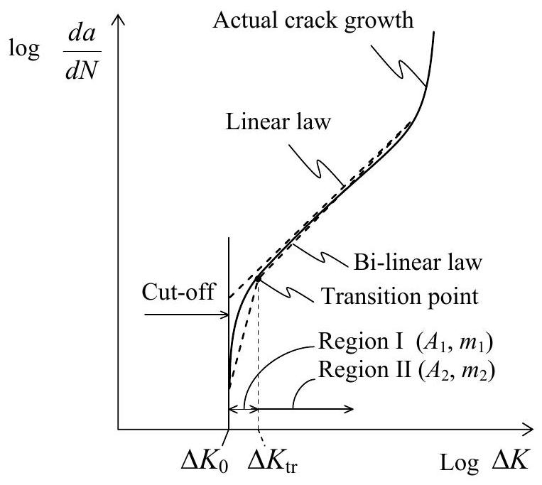
Fig. 34.1 Schematic representation of typical crack growth rates with linear and bi-linear approximations

The stress intensity factor \(K\) for a given applied (fluctuating) stress \(\sigma\) is given as:

(34.9)\[K=\sigma Y \sqrt{\pi a}\]

The stress \(\sigma\) should be determined from the applied loading in the vicinity of the crack location (but not influenced by the crack or the details of the weld). It does, however, include the stress concentration, resulting from the global geometry of the joint. The stress intensity correction factor \(Y\) depends on the crack size normalised with respect to other relevant local dimensions (e.g. plate thickness) and the nature of stress distribution. For details on \(Y\), see Annex A.

The through-thickness distribution of this stress is often assumed to consist of ‘membrane’ and ‘bending’ components and is characterised in terms of the ratio of the bending stress to the total stress, called ‘degree-of-bending’:

(34.10)\[K=\left(\sigma_{m} Y_{m}+\sigma_{b} Y_{b}\right) \sqrt{\pi a}\]

where the subscripts ‘ \(m\) ‘ and ‘ \(b\) ‘ refer to membrane and bending components respectively.

For welded joints micro-cracks often initiate from surface-breaking defects at the toe of the weld. These microcracks tend to coalesce to form a single, dominant fatigue crack of roughly semi-elliptical shape. Hence, semielliptical cracks in plated structures are of interest in many practical applications (Fig. 34.2). In this case, two crack dimensions, the depth \(a\) and the half-length at the surface \(c\), become relevant both of which are functions of the fatigue loading process.

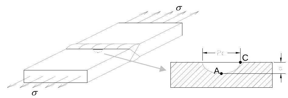
Fig. 34.2 A semi-elliptical crack in a steel plate at/near the weld toe

For each principal direction of crack growth a Paris type expression may be formulated,

(34.11)\[\begin{split}\begin{aligned} & \frac{d a}{d N}=A\left(\Delta K_{a}\right)^{m} \text { for } \Delta K_{a}>\Delta K_{0} \\ & \frac{d c}{d N}=A\left(\Delta K_{c}\right)^{m} \text { for } \Delta K_{c}>\Delta K_{0} \end{aligned}\end{split}\]

where the first expression relates to point \(\mathrm{A}\) and growth in the depth direction, whereas the second expression relates to point \(\mathrm{C}\) and growth in the length direction (see figure Fig. 34.2). For each of these points, the stress intensity factor range, \(\Delta K_{a}\) and \(\Delta K_{c}\), is given by

(34.12)\[\begin{split}\begin{aligned} & \Delta K_{a}=\Delta \sigma Y_{a} \sqrt{\pi a} \\ & \Delta K_{c}=\Delta \sigma Y_{c} \sqrt{\pi a} \end{aligned}\end{split}\]

where \(\Delta \sigma\) is the applied stress range and \(Y_{a}, Y_{c}\) are stress intensity correction factors for points \(\mathrm{A}\) and \(\mathrm{C}\) respectively.

Once equations (34.12) are substituted into (34.11), a pair of coupled differential equations is obtained. With the exception of the material parameters (\(A\) and \(m\) ) and the applied stress range \(\Delta \sigma\), all other terms are a function of the crack size \((a, c)\), which clearly changes during the fatigue loading process.

Limit state formulations

Using the fracture mechanics approach, the time dependent limit state function can be formulated as

(34.13)\[g(\boldsymbol{X}, t)=a_{c r}-a(t)\]

where \(\boldsymbol{X}\) is the vector of random variables, \(a_{c r}\) is a limiting crack depth (for example plate thickness) and \(a(t)\) is the crack depth after a service exposure of time \(t\). At \(t=0\) the crack size has an initial value \(a_{0}\). The calculation of the crack size at time \(t\) is not trivial as the stress is a random process. Assuming for \(\Delta \sigma\) a sufficiently mixing (ergodic) process we may use the expectation of the stress range to find the expectation of \(d a / d N\) (conditional upon the stress and fatigue model):

(34.14)\[\begin{split}\begin{aligned} E\left(\frac{d a}{d N}\right)= & A_{1} E\left[\Delta \sigma^{m_{1}}\right]_{\Delta \sigma_{0}}^{\Delta \sigma_{t r}}\left(C_{g l o b}~C_{s c f}~C_{s i f}~Y_{a}~\sqrt{\pi a}\right)^{m_{1}}+ \\ & +A_{2} E\left[\Delta \sigma^{m_{2}}\right]_{\Delta \sigma_{t r}}^{\infty}\left(C_{g l o b}~C_{s c f}~C_{s i f}~Y_{a}~\sqrt{\pi a}\right)^{m_{2}} \end{aligned}\end{split}\]

where \(C\) are model uncertainty factors for the various stress calculations (global analysis, stress concentration and stress intensity factor) and:

(34.15)\[E\left[\Delta \sigma^{m}\right]_{A}^{B}=\int_{A}^{B} s^{m} f_{\Delta \sigma}(s) d s\]

where \(f_{\Delta \sigma}(s)\) is the probability density function of the stress ranges \(\Delta \sigma\).

In general, the above integral is evaluated through an incremental numerical procedure, which involves subdivision of the total time into a number of steps. At each step, following the evaluation of equation (34.15) for the crack depth \(a\), the second crack dimension \(c\) is computed as well, using a similar set of equations. In that case, however, the value \(Y_{a}\) is replaced by \(Y_{c}\). As both \(a\) and \(c\) are simultaneously present in \(Y\), the two differential equations are coupled.

When the fatigue life of a fatigue sensitive detail is required, the critical crack size may for instance be taken as the plate thickness, but also as a critical value \(a_{cr}\) determined through the application of a fracture criterion. In that case the maximum crack size, \(a_{c r}\) that can be sustained by the component will depend on the material’s yield strength and fracture toughness \(K_{mat}\). The limit state function with respect to fracture can be formulated as:

(34.16)\[g(\mathbf{X}, t)=\min _{t} f\left(K_{r}, L_{r}\right)\]

where \(\boldsymbol{X}\) is the vector of random variables as a function of the time \(t, K_{r}\) is the fracture ratio, \(L_{r}\) is a measure of the proximity to plastic collapse and \(f()\) is an appropriate interaction criterion, as for example (see Fig. 34.3) given in [34.01] or (see Fig. 34.3) [34.03] as:

(34.17)\[f\left(K_{r}, L_{r}\right)=R-\sqrt{ }\left(K_{r}^{2}+L_{r}^{2}\right)\]

In this approach failure occurs when a stress cycle arrives that causes the reduced load bearing capacity of the cross section to be exceeded. The residual load bearing capacity depends on the actual crack size \(a\) and the interaction between the plastic and the brittle fracture failure modes. To evaluate the failure probability on the basis of (34.16) a time variant reliability method like the out-crossing approach is needed.

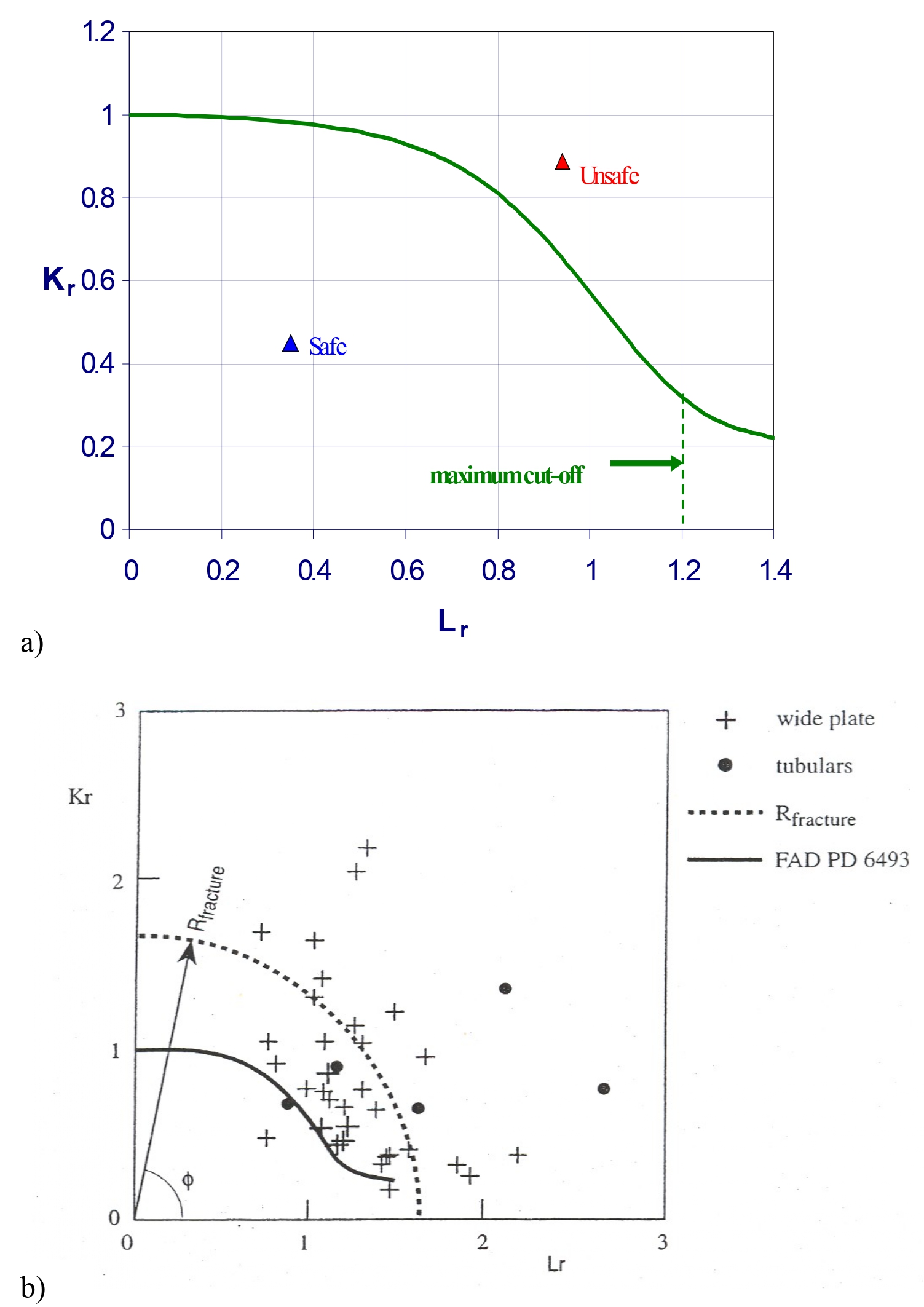
Fig. 34.3 \(K_{r}-L_{r}\) interaction curves according to [34.01] (above) and [34.03] (below)

In (34.17) the variable \(R\) is a normalised resistance parameter (nominally equal to 1.0) and the quantities \(K_{r}\) and \(L_{r}\) are defined as follows:

(34.18)\[K_{r}=\frac{K_{I}}{K_{m a t}}+\rho \text { and } L_{r}=\frac{\sigma_{n e t}}{\sigma_{y}}\]

where

\(K_{\text {mat }}\quad\) material toughness measured by stress intensity factor

\(K_{I} \quad\) stress intensity factor: \(K_{I}=(Y \sigma) \sqrt{\pi a}\)

\(\rho \quad\) plasticity correction factor

\(\sigma_{\text {net }}\quad\) net section stress (function of the crack size)

\(\sigma_{y} \quad\) yield stress

The factor \(\rho\) may be determined by the following procedure. For \(\chi=K_{I}^{s}~L_{r} / K_{I}^{p}>4\) an interpolating technique need to be applied (see [34.01]). For \(\chi \leq 4\) we have:

(34.19)\[\begin{split}\begin{array}{lll} \rho=\rho_{1} & \text { for } & L_{\mathrm{r}} \leq 0.8 \\ \rho=4 \rho_{1}\left(1.05-\mathrm{L}_{\mathrm{r}}\right) & \text { for } & 0.8<L_{r}<1.05 \\ \rho=0 & \text { for } & L_{\mathrm{r}} \geq 1.05 \end{array}\end{split}\]

with

(34.20)\[\rho_{1}=0.1 \chi^{0.714}-0.007 \chi^{2}+3 * 10^{-5} \chi^{5}\]

The crack size \(a\) may be determined from the fatigue crack growth models described above. The plasticity correction factor \(\rho\) reflects the interaction between the applied load (giving rise to the stress intensity factor \(K\)) and the residual stresses (giving rise to the stress intensity factor \(K_{I}^{S}\) ). Different residual stress profiles for various cracked geometries and restraint conditions may be assumed but their use implies that \(K_{I}^{s}\) would need to be evaluated using either finite element techniques or the weight function method. A simplified (and conservative) method would be to approximate the residual stress field via a linear stress field subtended from the surface and crack tip stress values. The corresponding \(K_{I}^{s}\) can then be obtained by superposition of the tensile and bending solutions for the geometry in question.

Further details of this approximation are given by [34.04]. If the bending solution is not known, in which case the previously mentioned procedure cannot be applied, the residual stress field may be assumed to be uniform. This approach will, in general, yield very conservative results for deep cracks and less conservative results for shallow cracks.

34.4. Probabilistic models

Table 34.1 gives an overview of all random variables and their probabilistic models. There are four blocks: one for the \(S-N\) parameters, one for the Fracture Mechanics parameters, one for the stress analysis and one for the Weibull stress process approximation. Additional commentary is given below:

\(S- N\) curve parameters

The stochastic model for the parameters in the \(S-N\)-based approach can be estimated as follows:

Step 1: For the fatigue detail considered, find (as good as possible) the corresponding detail and test data in the EC3 Background Document prEN 1993-1-9. RWTH, Aachen, 2002.

Step 2: Fit test data to a linear \(S-N\)-model: \(\log N=\log C-m \log \Delta \sigma+\varepsilon\) where \(N\) is the number of cycles to failure with stress range \(\Delta \sigma, \varepsilon\) is normally distributed with expected value 0 and standard deviation \(\sigma_{\varepsilon}\). The parameters \(\log C, m\) and \(\sigma_{\varepsilon}\) are fitted to the test data using the Maximum Likelihood Method including run-outs (no-failure tests) in the likelihood.

Step 3: The statistical uncertainty related to the parameter fits can be estimated using the Hessian of the Loglikelihhod function, and included in a reliability analysis.

A bilinear \(S-N\)-model can be fitted in a similar way. Usually \(m\) can be assumed fixed to 3 or 5 .

Miner’s sum at failure

Due to the random nature of fatigue damage, Miner’s damage sum at failure \(\left(D_{c r}\right)\) is not necessarily always exactly unity. It should therefore be treated as a random variable expressing the shortcomings of Miner’s rule. Wirsching (1984) suggests that \(D_{cr }\) be modelled as a lognormal variable with a mean of unity and coefficient of variation of 0.3 .

Crack growth parameters

When a simple Paris type crack propagation model is used, a random variable description for \(A\), is usually adequate. In this approach, the crack growth parameter \(A\) in the Paris law, can be used to describe the scatter in crack propagation data. The parameter \(A\) will in general depend on the applied stress ratio ( \(=\sigma_{\min } / \sigma_{\max }\) ) and the environmental conditions and is well described by a lognormal model with coefficient of variation typically in the range of 0.3 - 0.4. In the table the option to use a two branch model has been opened. For a one branch model one uses only \(m_{2}\) and \(A_{2}\). When a cut-off to crack growth \(\Delta K_{0}\) is adopted, \(\Delta K_{0}\) is lognormally distributed with a mean of \(140 \mathrm{Nmm}^{-3 / 2}\) and a coefficient of variation \(\mathrm{V}=0.4\) (Austen, 1983). In the case of freely corroding steels \(\Delta K_{0}=0\).

Initial defect size

The distribution of defect sizes should be based on defects existing in a structure entering service and includes those defects that are considered acceptable according to quality control standards, as well as those that remain undetected during fabrication. Thus defect occurrence rate, the amount and quality of NDE used, should be taken into account in developing a distribution for weld defect size. From the limited data available, the mean value and standard deviation of weld defect depth \(a_{0}\) can be estimated to be 0.15 mm and 0.10 mm for “sound” quality welds. Lognormal, exponential and Weibull distributions have been used by researchers to fit weld defect data. Similarly, initial defect aspect ratio, defined as the ratio of initial defect depth to defect semi-length ( \(a / c\) ) may also be modelled as a lognormal variable with a mean of 0.62 and coefficient of variation of 0.4 , Kountouris and Baker (1989).

Fatigue crack propagation model

The fatigue crack propagation model involves a number of parameters, which are subject to uncertainty. It is convenient to express all sources of uncertainty through a single basic variable \(C_{\text {sif }}\), which gives the ratio of stress intensity geometry factor obtained by experiment to that computed using the proposed model. The statistics for this variable can be developed by comparison with experimental compliance function curves. The factor \(C_{\text {sif }}\) can be modelled as a lognormal variable with a mean of unity and coefficient of variation typically in the range of 0.15 - 0.25. Lower variability may be used if the stress intensity factors are computed using finite element models such as line-spring and weight function models.

Fracture Toughness

For the fracture toughness \(K_{\text {mat }}\) a three-parameter Weibull distribution is proposed to describe fracture toughness related to cleavage fracture (Burdekin & Hamour, 2000; [34.05]; [34.06]):

(34.21)\[F_{K_{\text {mat }}}(k)=1-\exp \left[-\left(\frac{k-K_{0}}{\sigma}\right)^{\lambda}\right]\]

where

\(\lambda\) is the shape parameter, taken as 4 on the basis of experiments [34.07].

\(K_{0}\) is the threshold parameter, recommended is $20 \mathrm{MPa}~\mathrm{m}{ }^{1 / 2} {cite}BurdekinHamour2000`.

\(\sigma\) is the scale parameter and may be obtained from the following correlation attributed to Wallin [34.08]:

(34.22)\[\sigma=\left\lbrace 11+77\left[\exp \left(\frac{T-T_{27 J}+T_{0}}{52}\right)\right]\right\rbrace \left(\frac{25}{B}\right)^{1 / 4}\left(\mathrm{~K}_{\mathrm{mat}}\right. \text{in} \left.\mathrm{MPa}~\mathrm{m}{ }^{1 / 2}\right)\]

where:

\(T \quad\) operating temperature \(\left({ }^{\circ} \mathrm{C}\right)\) (random FBC process: \(\mu=10^{\circ} \mathrm{C}, \sigma=8^{\circ} \mathrm{C}, \Delta=10\) days)

\(T_{27 \mathrm{~J}} \quad\) temperature (\(\left({ }^{\circ} \mathrm{C}\right.\) ) corresponding to a \(\mathrm{CVN}\) of \(27 \mathrm{~J}\) (safe value)

\(T_{0} \quad\) temperature (random variability of \(\mathrm{T}_{27 \mathrm{~J}}: \mu=18^{\circ} \mathrm{C}, \sigma=15^{\circ} \mathrm{C}\) )

\(B \quad\) plate thickness in \([\mathrm{mm}]\)

\[ \text{Units:}~\mathbf{m m}~\text{and}~\mathbf{N} \]

Table 34.1 Probabilistic models for the random variables

Variable		Distribution	Mean	\(\mathbf{V}\)
\(C\)	Material parameter S-N curve	lognormal	\(1.0 \cdot 10^{13}\)	0.58
\(m\)	Slope value		3	-
\(\log C_{1}\)	Material parameter 2 par \(\mathrm{S}-\mathrm{N}\) curve	normal	Depends		\(C_{1}\) and \(C_{2}\) fully correlated
\(\log C_{2}\)	Material parameter 2 par \(\mathrm{S}-\mathrm{N}\) curve	normal	Depends		\(C_{1}\) and \(C_{2}\) fully correlated
\(m_{1}\) (air)	Slope value \(1^{\text {st }}\) branch	deterministic	5	-
\(m_{2}\) (air)	Slope value \(2^{\text {nd }}\) branch	deterministic	3	-
\(D_{c r}\)	Miner’s sum at failure	lognormal	1.0	0.3
\(A_{1}\) (air) \(^{*}\)	Paris Law Parameter 1	lognormal	\(4.80 \cdot 10^{-18}\)	1.70
\(A_{2}\) (air) \(^{*}\)	Paris Law Parameter 2	lognormal	\(5.86 \cdot 10^{-13}\)	0.60
\(m_{1}\) (air)	Slope value \(1^{\text {st }}\) branch	deterministic	5.10	-
\(m_{2}\) (air)	Slope value \(2^{\text {nd }}\) branch	deterministic	2.88	- -
\(\Delta K_{0}\) ( air )	Threshold value for \(\Delta K\)	lognormal	140	0.40
\(A_{1}\) (marine) \(^{*}\)	Paris Law Parameter 1	lognormal	\(5.37 \cdot 10^{-14}\)	1.10
\(A_{2}\) (marine) \(^{*}\)	Paris Law Parameter 2	lognormal	\(5.67 \cdot 10^{-7}\)	0.16
\(m_{1}\) (marine)	Slope value \(1^{\text {st }}\) branch	deterministic	3.42	- -
\(m_{2}\) (marine)	Slope value \(2^{\text {nd }}\) branch	deterministic	1.11	-
\(\Delta K_{0}\) (marine)	Threshold value for \(\Delta K\)	lognormal	0.0	- -
\(a_{0}\)	Initial crack depth	lognormal	0.15	0.66
\(a_{0} / c_{0}\)	Initial aspect ratio	lognormal	0.62	0.40
\(B_{\text {glob }}\)	MU global stress model \({ }^{*}\)	lognormal	1.0	0.10
\(B_{\text {scf }}\)	MU stress concentration	lognormal	1.0	0.20
\(B_{\text {sif }}\)	MU stress intensity factor (hand)	lognormal	1.0	0.20
\(B_{\text {sif }}\)	MU stress intensity factor (FEM)	lognormal	1.0	0.07
\(\sigma_{\text {res }}\)	Residual stresses	lognormal	300	0.20
\(R\)	Resistance fracture toughness	lognormal	1.7	0.18
\(K_{\mathrm{mat}}\)	Fracture toughness	Weibull	See (34.21)	See (34.21)

*stress ratio \(\sigma_{\min } / \sigma_{\max } \geq 0.5\)
\({ }^{* *} \mathrm{MU}=\) Model Uncertainty

34.5. Annex A: The stress intensity correction factor \(Y\)

The stress intensity correction factor \(Y\) for membrane loading is determined with the procedure of [34.09] and [34.01]. For the stress intensity correction factor in general they propose:

\[Y=M f_{w} M_{m} M_{k}\]

Factor \(M_{k}\) accounts for the local stress concentration and is provided in Annex A.2. The other factors are provided in Annex A.1. The resulting factors Ya and Yc (in height and width directions) are provided in Annex A.3

A1. The factors \(M, M_{m}\) and \(f_{w}\)

The equations and values provided below apply to membrane loading on flat plates with semi-elliptical cracks.

The factor \(M\) accounts for bulging effects. For flat plates, \(M=1\).

The finite-width correction function \(f_{w}\) is given by:

\[f_{w}=\left[\sec \left(\frac{\pi c}{W} \sqrt{\frac{a}{B}}\right)\right]^{1 / 2} \quad \text { for }(2 c / W) \leq 0.8\]

The stress intensity magnification factor for semi-elliptical cracks loaded in bending is equal to:

\[M_{m}=\left[M_{1}+M_{2}\left(\frac{a}{B}\right)^{2}+M_{3}\left(\frac{a}{B}\right)^{4}\right] g f_{\theta} / \Phi\]

Where:

\[M_{m}=\left[M_{1}+M_{2}\left(\frac{a}{B}\right)^{2}+M_{3}\left(\frac{a}{B}\right)^{4}\right] g f_{\theta} / \Phi\]

\[\begin{split} \begin{array}{ll} M_{1}=1.13-0.09(a / c) & \text { for } 0 \leq a / 2 c \leq 0.5 \\ \\ M_{1}=\sqrt{(c / a)}[1+0.04(c / a)] & \text { for } 0.5<a / 2 c \leq 1.0 \\ \\ M_{2}=\frac{0.89}{0.2+(a / c)}-0.54 & \text { for } 0 \leq a / 2 c \leq 0.5 \\ \\ M_{2}=0.2(c / a)^{4} & \text { for } 0.5<a / 2 c \leq 1.0 \\ \\ M_{3}=0.5-\frac{1.0}{0.65+(a / c)}+14[1.0-(a / c)]^{24} & \text { for } a / 2 c \leq 0.5 \\ \\ M_{3}=-0.11(c / a)^{4} & \text { for } 0.5<a / 2 c \leq 1.0 \\ \\ g=1+\left[0.1+0.35(a / B)^{2}\right](1-\sin \theta)^{2} & \text { for } a / 2 c \leq 0.5 \\ \\ g=1+\left[0.1+0.35(c / a)(a / B)^{2}\right](1-\sin \theta)^{2} & \text { for } 0.5<a / 2 c \leq 1.0 \end{array} \end{split}\]

The function \(f_{\theta}\), an angular function from the embedded elliptical-crack solution, is:

\[\begin{split} \begin{array}{ll} f_{\theta}=\left[(a / c)^{2} \cos ^{2} \theta+\sin ^{2} \theta\right]^{1 / 4} & \text { for } 0 \leq a / 2 c \leq 0.5 \\ f_{\theta}=\left[(c / a)^{2} \sin ^{2} \theta+\cos ^{2} \theta\right]^{1 / 4} & \text { for } 0.5<a / 2 c \leq 1.0 \end{array} \end{split}\]

The complete elliptic integral of the second kind \(\Phi\) is given by:

\[\begin{split} \begin{array}{ll} \Phi=\sqrt{1+1.464\left(\frac{a}{c}\right)^{1.65}} & \text { for } 0 \leq a / 2 c \leq 0.5 \\ \Phi=\sqrt{1+1.464\left(\frac{c}{a}\right)^{1.65}} & \text { for } 0.5<a / 2 c \leq 1.0 \end{array} \end{split}\]

The definitions of \(a, c\) and \(\theta\) are provided in Fig. 34.4.

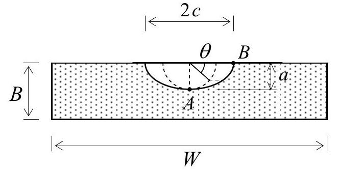
Fig. 34.4 Semi-elliptical crack geometry near weld toe

A2. The weld geometry factor \(M_{k}\)

The weld geometry \(M_{k}\) has to be incorporated if the crack is affected by a local stress concentration due to welding. The general formula is given by:

\[M_{k}=D(a / B)^{k 1}~(L / B)^{k 2} \qquad M_{k}>1\]

The parameters \(D\) and \(k\) depend on the structural and weld geometry as discribed by \(a, B\) and \(L\). For butt welds and X-joints a set of formulas for \(M_{\mathrm{ka}}\) values was derived by Maddox et al. (1986). These formulas are valid for weld toe angle \(\Theta=45^{\circ}\) and weld toe radius \(\rho=0\). The functions and the range of applicability are given in Table 34.2.

Table 34.2 Stress intensity concentration factors \((M_{\mathrm{ka}}\) ) for butt welds and X-joints

Loading mode	Applicability		Stress intensity concentration factor
	\(L / B\)	\(a / B\)	\(M_{\mathrm{ka}}=\mathrm{f}_{\mathrm{L}}(a / B, L / B)\)
axial	\(\leq 2\)	\(\leq 0.05(L / B)^{0.55}\)	\(0.51(L / B)^{0.27}(a / B)^{-0.31}\)
axial	\(\leq 2\)	\(>0.05(L / B)^{0.55}\)	\(0.83(a / B)^{-0.15(L / B)^{0.46}}\)
axial	\(>2\)	\(\leq 0.073\)	\(0.615(a / B)^{-0.31}\)
axial	\(>2\)	\(>0.073\)	\(0.83(a / B)^{-0.20}\)
bending	\(\leq 1\)	\(\leq 0.03(L / B)^{0.55}\)	\(0.45(L / B)^{0.21}(a / B)^{-0.31}\)
bending	\(\leq 1\)	\(>0.03(L / B)^{0.55}\)	\(0.68(a / B)^{-0.19(L / B)^{0.21}}\)
bending	\(>1\)	\(\leq 0.03\)	\(0.45(a / B)^{-0.31}\)
bending	\(>1\)	\(>0.03\)	\(0.68(a / B)^{-0.19}\)

\(a=\) crack depth, \(B=\) plate thickness and \(L=\) size of the node, defined acc. to Fig. 34.5.

For \(M_{\mathrm{kc}}\) we may use the same formulas, however substitute \(a=0,15 \mathrm{~mm}\) (See [34.01]).

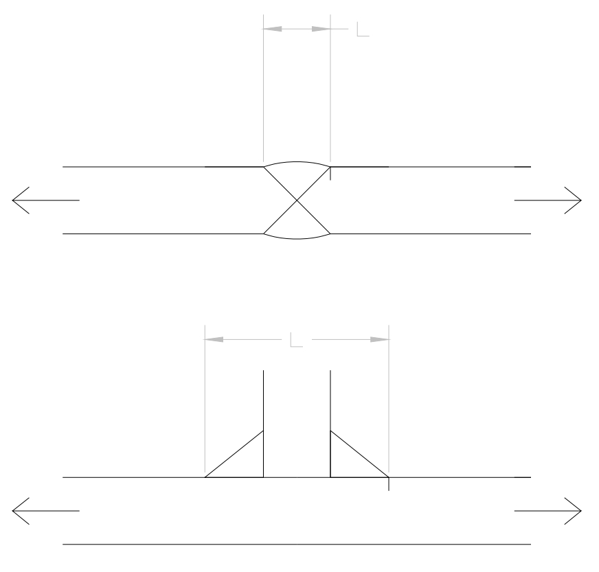
Fig. 34.5 Definition of node length L for two weld details

A3. The stress intensity correction factors \(Y_{a}\) and \(Y_{c}\)

For the factor \(Y_{a}\) it holds that \(\theta=\pi / 2\), therefore:

\[g=1 \quad ; \quad f_{\theta}=1 \text { for } 0 \leq a / 2 c \leq 0.5 \text { and } f_{\theta}=\sqrt{(c / a)} \quad\text { for } 0.5<(a / 2 c) \leq 1.0\]

For \(Y_{c}\) with \(\theta=0\) it follows:

\[g=1.1+0.35(a / \mathrm{B})^{2} ; \quad f_{\theta}=\sqrt{a / c} \quad \text { for } 0 \leq a / 2 c \leq 0.5 \quad \text { and } \quad f_{\theta}=1 \quad \text { for } 0.5<(a / 2 c) \leq 1.0\]

Both factors finally become:

\[\begin{split}\begin{array}{ll} Y_{a}=M_{k a}\left[M_{1}+M_{2}\left(\frac{a}{B}\right)^{2}+M_{3}\left(\frac{a}{B}\right)^{4}\right] f_{w} / \Phi & \text { for } 0 \leq a / 2 c \leq 0.5 \\ Y_{a}=M_{k a}\left[M_{1}+M_{2}\left(\frac{a}{B}\right)^{2}+M_{3}\left(\frac{a}{B}\right)^{4}\right] f_{w} \sqrt{(c / a)} / \Phi & \text { for } 0.5<(a / 2 c) \leq 1.0 \\ Y_{c}=M_{k c}\left[M_{1}+M_{2}\left(\frac{a}{B}\right)^{2}+M_{3}\left(\frac{a}{B}\right)^{4}\right] f_{w}\left\lbrace 1.1+0.35(\mathrm{a} / \mathrm{B})^{2}\right\rbrace \sqrt{(c / a)} / \Phi & \text { for } 0 \leq a / 2 c \leq 0.5 \\ Y_{c}=M_{k c}\left[M_{1}+M_{2}\left(\frac{a}{B}\right)^{2}+M_{3}\left(\frac{a}{B}\right)^{4}\right] f_{w}\left\lbrace 1.1+0.35(\mathrm{a} / \mathrm{B})^{2}\right\rbrace / \Phi & \text { for } 0.5<(a / 2 c) \leq 1.0 \end{array}\end{split}\]

34.6. Appendix B: Fatigue Loading evaluation

In the \(S-N\) approach as well as in the Fracture Mechanics approach the loading term contains the expectation of the \(m^{\text {th }}\) moment of the (ergodic part) of the stress distribution.

B1 Narrow band

Rayleigh distribution

If the stress spectrum is Gaussian and narrow-banded it can be shown that the peaks of the stress process, and hence the stress ranges, follow a Rayleigh distribution. For this case the \(m^{\text {th }}\) moment of the stress range density function can be obtained as:

\[E\left[\Delta S^{m}\right]=(2 \sigma \sqrt{2})^{m} \Gamma\left(\frac{m}{2}+1\right)\]

where \(\sigma\) is the standard deviation of the stress process and \(\Gamma()\) is the Gamma function.

In case we have S-N-lines or fracture mechanics models with two branches:

\[\begin{split}\begin{aligned} & E\left(\Delta S^{m}\right)_{0}^{S o}=(2 \sigma \sqrt{2})^{m 1} \Gamma\left(\frac{m_{1}}{2}+1 ;\left(\frac{S_{0}}{2 \sigma \sqrt{2}}\right)^{2}\right) \\ & E\left(\Delta S^{m}\right)_{S o}^{\infty}=(2 \sigma \sqrt{2})^{m 2} \Gamma_{o}\left(\frac{m_{2}}{2}+1 ;\left(\frac{S_{0}}{2 \sigma \sqrt{2}}\right)^{2}\right) \end{aligned}\end{split}\]

Two parameter Weibull distribution

Assume that the stress ranges are Weibull distributed with distribution function:

\[F_{\Delta s}(s)=1-\exp \left(-\left(\frac{s}{k}\right)^{\lambda}\right)\]

In that case we have for the stress expectations

\[E\left(\Delta S^{m}\right)=k^{m} \Gamma\left(\frac{m}{\lambda}+1\right)\]

In case we have S-N-lines or fracture mechanics models with two branches:

\[\begin{split}\begin{aligned} & E\left(\Delta S^{m}\right)_{0}^{S o}=k^{m 1} \Gamma\left(\frac{m_{1}}{\lambda}+1 ;\left(\frac{S_{0}}{k}\right)^{\lambda}\right) \\ & E\left(\Delta S^{m}\right)_{S o}^{\infty}=k^{m 2} \Gamma_{o}\left(\frac{m_{2}}{\lambda}+1 ;\left(\frac{S_{0}}{k}\right)^{\lambda}\right) \end{aligned}\end{split}\]

Where \(\Gamma(a ; b)\) denotes the Incomplete Gamma function and \(\Gamma_{0}(a ; b)=\Gamma(a)-\Gamma(a ; b)\) the complementary Gamma function

Note that the Rayleigh distribution for the stress ranges corresponds to a Weibull distribution with \(\lambda=2\) and \(\mathrm{k}=2 \sigma \sqrt{ } 2\), where \(\sigma\) is the standard deviation of the underlying Gaussian stress process.

B2 Broad banded processes:

When the stress process is broad-banded, the stress cycles cannot be easily distinguished, and a convention is required for defining stress cycles. Broadly, there are two approaches available for the modelling of stress cycles of a broad-banded stress process:

Cycle Counting Methods

The first approach is to simulate the time history of the stress process and use one of the peak, range or rain flow counting schemes to count the stress cycles, see Dowling (1972). The rain flow counting method is seen to give a good correlation with experimental results of fatigue tests under variable amplitude loading.

Semi-Analytical Probability Distributions

In the second approach, analytical distributions for stress ranges of a wide banded stress process are derived empirically, like the following 5-parameter mixed Weibull distribution by Zhao and Baker (1990):

\[\begin{split}\begin{aligned} & f_{Y}(y)=\gamma \frac{b_{w}}{a_{w}}\left(\frac{y}{a_{w}}\right)^{b_{w}-1} \exp \left[-\left(\frac{y}{a_{w}}\right)^{b_{w}}\right]+(1-\gamma) \frac{d_{w}}{c_{w}}\left(\frac{y}{c_{w}}\right)^{d_{w}-1} \exp \left[-\left(\frac{y}{c_{w}}\right)^{d_{w}}\right] \\ & a_{w}=(8-7 \alpha)^{-1 / b} \\ & b_{w}=1.1 \quad \text { for } \quad \alpha \leq 0.9 \\ & b_{w}=1.1+9(\alpha-0.9) \quad \text { for } \quad \alpha>0.9 \\ & c_{w}=\sqrt{2} \\ & d_{w}=2 \\ & \alpha=\frac{m_{2}}{\sqrt{m_{0} m_{4}}} \\ & \gamma=\frac{1-\alpha}{1-\sqrt{2 / \pi} a_{w} \Gamma\left(\frac{1}{b_{w}}+1\right)} \end{aligned}\end{split}\]

where \(y=\Delta S / 2 \sigma\) is the normalised stress range and \(\sigma\) is the standard deviation or ‘root mean squared’ (rms) value of the stress process; \(m_{0}, m_{2}\) and \(m_{4}\) are the zero, second and fourth moment of the stress process.

For this distribution the \(m^{\text {th }}\) expected value of stress range \(E\left[y^{m}\right]\) can be calculated:

\[E\left[y^{m}\right]=\gamma a_{w}^{m}~\Gamma\left(\frac{m+b_{w}}{b_{w}} ; y_{t h}\right)+(1-\gamma) c_{w}^{m}~\Gamma\left(\frac{m+d_{w}}{d_{w}} ; y_{t h}\right) \quad ; \quad y_{t h}=\frac{S_{t h}}{2 \sigma}\]

where \(\Gamma(\cdots ; \cdots)\) is the incomplete Gamma function. When the expectation is over all stress cycles, this can be replaced by the complete Gamma function in the above expressions. In fracture mechanics \(S_{t h}\) is defined in terms of the stress range corresponding to \(\Delta K_{t h}\) via Eq (34.12) and can be seen as a function of the random crack depth \(a\) and random aspect ratio \(a / c\). In the case of an S-N approach, the threshold may refer to some nonpropagating stress or cut off value.

References

[34.01] (1,2,3,4,5,6)

British Standards Institution. Bs7910: guide on methods for assessing the acceptability of flaws in fusion welded structures. Standard, British Standards Institution, London, 2000.

[34.02]

P.C. Paris and F.A. Erdogan. A critical analysis of crack propagation laws. J. Basic Engineering, 1963.

[34.03] (1,2)

O.D. Dijkstra and others. A fracture mechanics approach to the assessment of the remaining fatigue life of defective welded joints. In IABSE Workshop. Lausanne, April 1991. 1990.

[34.04]

H. Tada, P.C. Paris, and G.R. Irwin. The stress analysis of cracks handbook. ASME, New York, 2000.

[34.05]

M. Lukić and C. Cremona. Probabilistic assessment of welded joints versus fatigue and fracture. J. Struct. Engg., 2001.

[34.06]

T.D. Righiniotis and M.K. Chryssanthopoulos. Probabilistic fatigue analysis under constant amplitude loading. Journal of Constructional Steel Research, 59(7):867–886, 2003.

[34.07]

K. Wallin. The scatter in k kc results. Eng. Fract. Mechs., 1984.

[34.08]

F.M. Burdekin and W. Hamour. Partial safety factors for sintap procedure. Technical Report, Offshore Technology Report, OTO 2000 020, HSE, London, 2000.

[34.09]

J.C. Newman and I.S. Raju. An empirical stress intensity factor equation for the surface crack. Engg. Fract. Mechs., 1981.

Additional References

1. Hobbacher, A. (1993). “Stress intensity factors of welded joints”, Eng. Fract. Mech., Vol. 46(2).

2. Newman, J.C. and Raju, I.S. (1986). “Stress-intensity factor equations for cracks in three-dimensional finite bodies subjected to tension and bending loads”, Computational Methods in the Mechanics of Fracture, S.N. Atluri (ed), Elsevier North Holland, New York.

3. Righiniotis, T.D. and Chryssanthopoulos, M.K. (2004). “Fatigue and fracture simulation of welded bridge details through a bi-linear crack growth law”, Struct. Safety, Vol. 26.

4. Shetty, N.K. and Baker, M.J. (1990). “Fatigue reliability of tubular joints in offshore structures: Crack propagation model”, Proc. 9th Offshore Mechanics and Arctic Engineering Conf., ASME.