
23. General Principles#
List of symbols:
\(\begin{array}{ll}f_{x}(x \mid q) &= \text { the variability of property} x \text { within a given lot}\\ f_{q}(q) &= \text { the variability of the parameters}~q \text { from lot to lot; statistical description of the production}\\ f^{\prime}(q) &= \text { prior distribution of}~q\\ f^{\prime \prime}(q) &= \text { posterior distribution of}~q\\ L (\text { data} \mid q) &= \text { likelihood function}\\ q &= \text { vector of distribution parameters (e.g. mean and std. dev.)}\\ C &= \text { normalising constant}\\ d &= \text { decision rule}\end{array}\)
23.1. Introduction#
The description of each material property consists of a mathematical model (e.g. elastic-plastic model, creep model, etc.) and random variables or random fields (e.g. modulus of elasticity, creep coefficient). Functional relationships between the various variables may be part of the material model (e.g. the relation between tensile stress and compressive stress for concrete).
In general, it is the response to static and time dependent mechanical loading that matters for structural design. However, also the response to physical, chemical and biological actions is important as it may affect the mechanical properties and behaviour.
It is understood that modelling is an art of reasonable simplification of reality such that the outcome is sufficiently explanatory and predictive in an engineering sense. An important aspect of an engineering model is also its operationability, i.e. the ease in handling it in applications.
Models and values should follow from (standardised) tests, representing the actual environmental and loading conditions as good as possible. The set of tested specimen should be representative for the production of the relevant fabrication sites, cover a sufficient long period of time and may include the effect of standard quality control measures. Allowance should be made for possible differences between test circumstances and structural environment (conversion).
For the classical building materials, knowledge about the various properties is generally available from experience and from tests in the past. For new materials, models and values should be obtained from an extensive and well defined testing program.
23.2. Material properties#
Material properties are defined as the properties of material specimens of defined size and conditioning, sampled according to given rules, subjected to an agreed testing procedure, the results of which are evaluated according to specified procedures.
The main characteristics of the mechanical behaviour is described by the one dimensional \(\sigma-\varepsilon-\) diagram, as presented in Fig. 23.1. As an absolute minimum for structural design the
modulus of elasticity
the strength of the material
both for tensile and compression should be known. Other important parameters in the one-dimensional \(\sigma-\varepsilon-\) diagram are:
yield stress (if present)
limit of proportionality
strain at rupture and strain at maximum stress
The strain at rupture is a local phenomenon and the value obtained may heavily depend on the shape and dimensions of the test specimen.
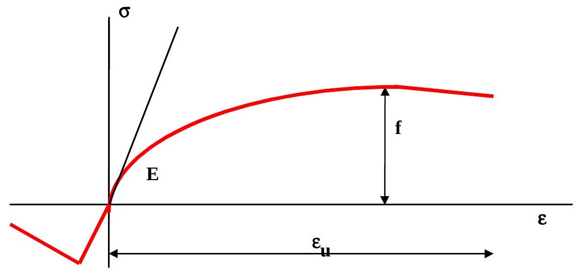
Fig. 23.1 Stress strain relationship#
Additional to the one dimensional \(\sigma-\varepsilon-\) diagram, information about a number of other quantities and effects is of importance, such as:
Multi-axial stress condition
Duration and strain rate effects
Temperature effects
Humidity effects
Effects of notches and flaws
Effects of chemical influences
In general, the various properties of one material may be correlated.
In the present version of this JCSS model code not all properties will be considered.
23.3. Uncertainties in material modelling#
Material properties vary randomly in space: The strength in one point of a structure will not be the same as the strength in another point of the same structure or another one. This item will be further developed in the sections 23.4. and 23.5..
Additional to spatial variations of materials, the following uncertainties between measured properties of specimen and properties of the real structure should be accounted for.
Systematic deviations identified in laboratory testing by relating the observed structural property to the predicted property, suggesting some bias in prediction.
Random deviations between the observed and predicted structural property, generally suggesting some lack of completeness in the variables considered in the model.
Uncertainties in the relation between the material incorporated in the structural sample and the corresponding material samples.
Different qualities of workmanship affecting the properties of (fictitious) material samples, i.e. when modelling the material supply as a supply of material samples.
The effect of different qualities of workmanship when incorporating the material in actual structures, not reflected in corresponding material samples.
Uncertainties related to alterations in time, predictable only by laboratory testing, field observations, etc.
23.4. Scales of modelling variations#
Material properties vary locally in space and, possibly, in time. As far as the spacial variations are concerned, it is useful to distinguish between three hierarchical levels of variation: global (macro), local (meso) and micro (see Table 23.1).
For example, the variability of the mean and standard deviation of concrete cylinder strength per job or construction unit as shown in Fig. 23.2 is a typical form of global parameter variation. This variation primarily is the result of production technology and production strategy of the concrete producers. Parameter variations between objects are conveniently denoted as macroscale variations. The unit of that scale is in the order of a structure or a construction unit. Parameter variations may also be due to statistical uncertainties.
Given a certain parameter realisation in a system the next step is to model the local variations within the system in terms of random processes or fields. Characteristically, spatial correlations (dependencies) become negligible at distances comparable to the size of the system. This is a direct consequence of the hierarchical modelling procedure where it is natural to assume that the variation within the system is conditional on the variations between systems and the first type of variation is conditionally independent of the second. At this level one may speak of meso-scale variations. Examples are the spatial variation of soils within a given (not too large) foundation site or the number, size and spatial distribution of flaws along welding lines given a welding factory (or welding operator). The unit of this scale is in the order of the size of the structural elements and probably most conveniently measured in meters.
At the third level, the micro-level, one focuses on rapidly fluctuating variations and inhomogenities which basically are uncontrollable as they originate from physical facts such as the random distribution of spacing and size of aggregates, pores or particles in concrete, metals or other materials. The scale of these variations is measured in particle sizes, i.e. in centimeters down to the size of crystals.
The modelling process normally uses physical arguments as far as possible. Quite generally, the object is taken as an arrangement of a large number of small elements. The statistical properties of these elements usually can only be assessed qualitatively as well as their type of interaction. This, however, is sufficient to perform some basic operations such as extreme value, summation or intersection operations which describe the overall performance. The large number of elements greatly facilitates such operations because one can make use of certain limit theorems in probability theory. The advantage of using asymptotic concepts rests on the fact that the description of the element properties can then be reduced to some few essential characteristics. The central limit theorem of probability theory, asymptotic extreme value concepts, convergence theorems to the Poisson distribution, etc. will play an important role. In particular, size effects have to be taken into account at this level.
A useful concept is to introduce a reference volume of the material which in general is chosen on rather practical grounds. It most frequently corresponds to some specified test specimen volume at which material testing is carried out. This volume generally neither corresponds to the volume of the virtual strength elements introduced at the micro-scale modelling level nor to a characteristic volume for in situ strength. It eds to be related to the latter one and these operations can involve not only simple size scaling but more complicated functional relationships if the material produced is subject to further uncertain factors once put in place. Concrete is the most obvious example for the necessity of such additional consideration. Of course, scale effects may also be present at the meso-scale level of modelling.
The reason for this concept of modelling at several levels (steps) is the requirement for operationability not only in the probabilistic manipulations but also in sampling, estimation and quality control. This way of modelling and the considerations below are, of course, only valid under certain technical standards for production and its control. At the macro-scale level it is assumed that the production process is under control. This simply means that the outcome of production is stationary in some sense. Should a trend develop, production control corrects for it immediately or with some sufficiently small delay. Therefore, it is assumed that at least for some time interval (or spatial region) whose length (size) is to be selected carefully, approximate stationarity on the meso- and micro-scale is guaranteed. Quite frequently, the operational, mathematical models available so far even require ergodicity. Variations at the macro scale level, therefore, can be described by stationary sequences. If the sequences are or can be assumed independent, it is possible to handle macro-scale variations by the concept of random variables. Stationarity is also assumed at the lower levels. However, it may be necessary to use the theory of random processes (fields) at the lower levels, especially in order to take into account of significant effects of dependencies in time or space.
23.5. Hierarchical modelling#
Consider a random material property \(X\) which is described by a probability density function \(f_{x}(x \mid \mathbf{q})\), where \(\mathbf{q}=\left(q_{1}, q_{2}, \ldots\right)\) is the statistical parameter vector, e.g. \(q_{1}\) is the mean and \(q_{2}\) the standard deviation. The density function \(f_{x}(x \mid \mathbf{q})\) applies to the property of a finite reference volume, identical with or clearly related to the volume of the test specimen within a given unit of material. Guidance on the type of distribution may be obtained by assessing the performance of the reference volume under testing conditions in terms of some micro system behaviour. The performance of test specimens, regarded as a system of micro elements, can usually be interpreted by one of the following strength models
Weakest link model
Full plasticity model
Daniel’s bundle of threads model
When applying these models to systems with increasing number of elements, they generally lead to specific distributions for the properties of the system at the meso-scale level. The weakest link model leads to a Weibull distribution, the other two models to a normal distribution. For larger coefficients of variation the normal distribution must be replaced by a lognormal distribution in order to avoid physically impossible, negative strength values.
In the next step (see Table 23.1) a unit (a structural member) is considered as meso-scale (local variations). The respective unit is regarded as being constituted from a sequence of finite volumes. Hence, a property in this unit is modelled by a random sequence \(X_{1}, X_{2}, X_{3} \ldots\) of reference volume properties. The \(X_{i}\) may have to be considered as correlated, with a coefficient of correlation depending on the distance \(\Delta r_{ij}\) and a correlation parameters \(\rho_{o}\) and \(d_{c}\), for example:
In general \(\rho_{0}=0\).
In the subsequent step the complete structure or some relevant part of it is considered as a lot. A lot is defined as a set of units, produced by one producer, in a relatively short period, with no obvious changes in production circumstances and intended for one building site. In practice lots correspond to e.g.:
the production of ready-mix concrete for a set of elements
structural steel from one melt processed according to the same conditions
foundation piles for a specific site
As a lot is a set of units it can also be conceived as a set of reference volumes \(X_{i}\). Normally the parameters \(q\) defined before are defined on the lot level. The correlation between the \(X_{i}\) values within different members normally can be modelled by a single parameter
Finally, at the highest macro scale level, we have a sequence of lots, represented by a random sequence of lot parameters (in space or in time). Here we are concerned with the estimation of the distribution of lot parameters, either from one source or several sources. The individual lots may be interpreted as random samples taken from the enlarged population or gross supply. The gross supply comprises all materials produced (and controlled) according to given specifications, within a country or groups of countries. The macro-scale model may be used if the number of producers and structures is large or differences between producers can be considered as approximately random.
Scale |
Population |
Reference name |
Description |
|---|---|---|---|
macro (global) |
set of structures |
gross supply |
\(\mathbf{X}\) |
meso |
set of elements |
lot |
\(\mathbf{X} \mid \mathbf{q}\) and \(\boldsymbol{\rho}_{\mathbf{o}}\) |
meso (local) |
one element |
unit |
\(\mathbf{X} \mid \mathbf{q}\) and \(\boldsymbol{\rho}(\Delta \mathbf{r})\) |
micro |
aggregate level |
reference volume |
type of distribution |
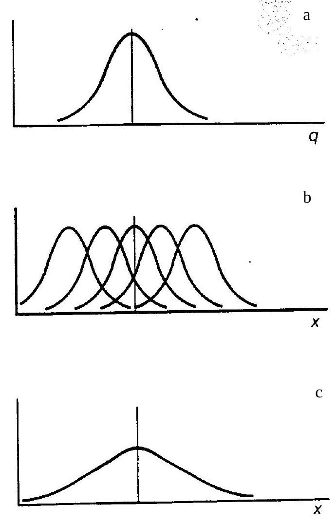
Fig. 23.2 Figure a) production description \(\mathrm{f}_{\mathrm{q}}(\mathrm{q})\)#
Figure b) lot description \(\mathrm{f}_{\mathrm{x}}(\mathrm{x} \mid \mathrm{q})\)
Figure c) total supply \(\mathrm{f_{x}(x)}\)
Description of production parameters, lots and total supply
The gross supply is described by \(f(q)\). Type and parameters should follow from a statistical survey of the fluctuations of the various lots which belong to the production under consideration. It will be assumed here that \(f(q)\) is known without statistical uncertainty. If statistical uncertainties cannot be neglected, they can be incorporated. The distribution \(f(q)\) should be monitored more or less continuously to find possible changes in production characteristics.
The probability density function (predictive density function) for an arbitrary unit (arbitrary means that the lot is not explicitly identified) can be found from the total probability theorem:
The density function \(f(x)\) may be conceived as the statistical description of \(x\) within a large number of randomly selected lots. For some purposes one could also identify \(f(x)\) directly.
23.6. Definition of characteristic value#
The characteristic value of a material with respect to a given property \(X\) is defined as the \(p_{x}\) - quantile in the predictive distribution, i.e.
Examples for predictive distributions can be found in Annex A. Others may be found in [23.01], [23.02] and [23.03].
23.7. Quality control strategies#
23.7.1. Types of strategies#
Normally the statistical parameters of the material properties are based on general tests, taking into account standard production methods. For economic reasons it might be advantageous to have more specific forms of quality control for a particular work or a particular factory.
Quality control may be of a total (all units are tested) or a statistical nature (a sample is tested). Quality control will lead to more economical solutions, but has in general the disadvantage that the result is not available at the time of design. In those cases, the design value has to be based on the combination of the unfiltered production characteristics and the expected effect of the quality control selection rules.
Various quality control procedures can be activated, each one leading to a different design value. In Fig. 23.3 an overview is presented. The easiest procedure is to perform no additional activities (option “no tests”). This means that the units, lots, production should be defined, their descriptions \(f(x \mid q)\) and \(f(q)\) should be established and only \(f(q)\) should be checked for long term changes in production characteristics.
If on the other hand tests are performed one may distinguish between a total (unit by unit) control and sampling on the one hand and between selection and updating on the other hand. The various options will be discussed.
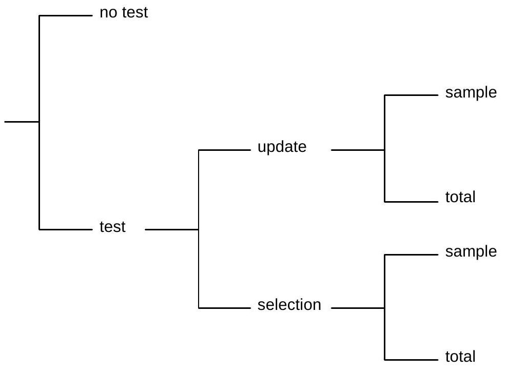
Fig. 23.3 Strategies for Quality Control#
23.7.2. Total testing versus Sampling#
Both for updating and for selection one may test all units which go into a structure (total testing) or one may test a (random) sample only (statistical testing).
If the control is total, every produced unit is inspected. The acceptance rules imply that a unit is judged as good (accepted) or bad (not accepted). This type of control is also referred to as unit by unit control. Typically, testing all units requires a non-destructive testing technique. Therefore some kind of measurement error has to be included resulting in a smooth truncation of the distribution.
If the control is statistical only a limited member of units is tested. The procedure generally consists of the following parts:
batching the products;
sampling within each lot;
testing the samples;
statistical judgement of the results;
decision regarding acceptance.
One normally takes a random sample. In a random sample each unit of the lot has the same probability of being sampled. Where knowledge on the inherent structure of the lot is available, this could be utilised, rendering more efficient sampling techniques, e.g.:
sampling at weak points, when trends are known;
sampling at specified intervals;
stratified sampling;
The larger efficiency results in smaller sample sizes for obtaining the same filtering capability of a test. No further guidance, however, will be given here.
23.7.3. Updating versus selecting#
Testing can be done with two purposes:
to update the probability density function \(f(x)\) or \(f(q)\) of some particular lot or item (updating);
to identify and reject inadequate lots or units on the basis of predefined sampling procedures and selection rules (selection).
The basic formula for the first option is given by:
where:
\(f^{\prime \prime}(q) =\) posterior distribution of q
\(f^{\prime}(q) =\) prior distribution of q
\(L(\text { data/q }) =\) likelihood of the data
\(q =\) vector of distribution parameters (e.g. mean and std. dev.)
\(C =\) normalising constant = \(\int L(\text { data } \mid q) f^{\prime}(q) d q\)
For the normal case more detailed information is presented in Annex A.
The first option can only be used after production of the lot or item under consideration. This data may not be known at the time of the design (e.g. ready mix concrete). The second option, on the other hand, offers the possibility to predict the posterior \(f^{\prime \prime}(q)\) for the filtered supply for a given combination of \(f(x \mid q), f(q)\) and a selection rule \(d\). In such a case the control may lead to two possible outcomes:
the lot (or unit) is rejected \(\qquad: d \notin A\)
the lot (or unit) is accepted \(\qquad: d \in A\)
Here \(d\) is a function of the test result of a single unit or of the combined test result of the units in a sample and \(A\) is the acceptance domain.
One may then calculate the posterior distributions for an arbitrary accepted lot:
Here \(f(q)\) is the distribution function for the unfiltered supply and the acceptance probability \(P(d \in A \mid q)\) should be calculated from the decision rule.
The updated distribution for \(X\) can be obtained through (23.3) with \(f(q)\) replaced by \(f^{\prime \prime}(q)\).
More information about the effect of quality cobntrol on the distribution of material properties can be found in [23.04].
23.8. Annex A: Bayesian evaluation procedure for the normal and lognormal distribution - characteristic values#
If \(X\) has a normal distribution with parameters \(q_{1}=\mu\) and \(q_{2}=\sigma\) it is convenient to assume a prior distribution for \(\mu\) and \(\sigma\) according to:
\(k=\) normalizing constant
\(\delta\left(n^{\prime}\right)=\) 0 for \(n^{\prime}=0\)
\(\delta\left(n^{\prime}\right)=\) for \(n^{\prime}>0\)
This special choice enables a further analytical treatment of the various operations. The prior distribution (23.7) contains four parameters: \(m^{\prime}, n^{\prime}, s^{\prime 2}\) and \(v^{\prime}\).
Using equation (23.4) one may combine the prior information characterised by (23.7) and a test result of \(n\) observations with sample mean \(m\) and sample standard deviation \(s\). The result is a posterior distribution for the unknown mean and standard deviation of \(X\), which is again given by (23.7), but with parameters given by the following updating formula’s:
Then, using equation (23.3) the predictive value of \(X\) can be found from:
where \(t_{v^{\prime \prime}}\) has a central t-distribution.
In case of known standard deviation \(\sigma\) eq. (23.2) and (23.4) still hold for the posterior mean. The predictive value of \(X\) is
where \(u\) has a standard normal distribution.
The characteristic value is thus defined as
For \(n^{\prime \prime} v^{\prime \prime} \rightarrow \infty~~x_{c}=m^{\prime \prime} + u\left(p_{x}\right) s^{\prime \prime}\) in both cases with \(s^{\prime \prime}=\sigma\).
If \(X\) has a lognormal distribution, \(Y=\ln (X)\) has a normal distribution. One may then use the former formula’s on \(Y\) and use \(X=\exp (Y)\) for results on \(X\).
23.9. Annex B: Bayesian evaluation procedure for regression - characteristic value#
If only indirect measurements for the quantity of interest are possible and a linear regression model \(y=a_{0}+a_{1} x\) is suitable the predictive value of \(y\) has also a t-distribution given by
where
\(a_{0}=\bar{y}-a_{1} \bar{x}\)
\(a_{1}=\frac{\sum_{i=1}^{n} x_{i} y_{i}-n \overline{x y}}{\sum_{i=1}^{n} x_{i}^{2}-n \bar{x}^{2}}\)
\(\bar{x}=\frac{1}{n} \sum_{i=1}^{n} x_{i}\)
\(\bar{y}=\frac{1}{n} \sum_{i=1}^{n} y_{i}\)
\(s^{2}=\frac{1}{n-2} \sum_{i=1}^{n} \left(y_{i}-a_{0}-a_{1} x_{i} \right)^2\)
\(v=n-2\)
The characteristic value corresponding to the quantile \(p\) is
For example, for S-N curves, it is \(y=\ln (N), x=\ln (\Delta \sigma), a_{1}=-m\) and \(a_{0}=\ln a\). The characteristic value of \(N\) for given \(\ln \left(\Delta \sigma_{E}\right)=x_{0}\) is \(N_{c}=\exp \left[y_{c}\right]\).
References
J. Aitchison and I.R. Dunsmore. Statistical Prediction Analysis. Cambridge University Press, Cambridge, 1975.
H. Raiffa and R. Schlaifer. Applied Statistical Decision Theory. MIT Press, Cambridge, 1968.
S. Engelund and R. Rackwitz. On predictive distribution functions for the three asymptotic extreme value distributions. Structural Safety, 11:255–258, 1992.
M. Kersken-Bradley and R. Rackwitz. Stochastic modeling of material properties and quality control. JCSS Working Document, Joint Committee on Structural Safety, March 1991. IABSE-publication.